Is there an open-source alternative to Suno in 2026?
Every couple of weeks, another open-source ai music generator model launches with a headline claiming Suno parity. Sometimes it is the abstract, sometimes a benchmark table column, sometimes a curated thread on X, but the claim is always the same: the open community has caught up. We went looking for independent head-to-head comparisons and could not find enough good material. We get asked about open-weights song generation often enough that we wanted somewhere honest to point. So we ran the comparison ourselves, on the May 2026 slate of models we could load and run.
The short answer: no, there is not an open-source Suno yet. The closest model, by our ears, gets within audible-but-real distance of Suno V5 on some prompts and trails on others; everything else trails further. DiffRhythm 2 makes the same call in its own paper: “Open-source still falls short of commercial systems overall.” 🔗. We agree. The rest of this post is the longer version of why.
There is no single open winner across all the things you might care about.
- The model that produced the most natural-sounding music carries a non-commercial license.
- The model best suited to research, fine-tuning, and continued experimentation is permissively licensed but has audible artifacts.
A third model in the set is the most architecturally distinctive thing released in 2026 and currently ships with a stability disclaimer from the authors themselves. Roughly: the model that wins on quality wins at a license cost, and the model that wins on freedom and tooling wins at an audio cost. Which compromise is the right one depends on what you are trying to build, and the rest of the post walks through that trade-off model by model.
Want to skip straight to the audio comparison? Jump to the listening table.
There has been a real wave of strong work in this space. The engineering behind several of the 2026 releases is substantial, and we will say so when we get to them. But the announcement layer makes that wave hard to read honestly: launch posts cherry-pick the best seeds, comparison tables come from the teams who also publish models, demo reels are curated, every release claims to be state of the art on a benchmark its own authors built. After enough cycles of this, even experienced readers stop trusting the headlines and start downloading the weights themselves, which is expensive in time. We did that work, on the cheaper kind of cloud GPU, on the same three style-and-lyric combinations across every model. The post is for the reader who would otherwise have to do it: product leads weighing whether song generation belongs in something they’re building, musicians evaluating tools, engineers choosing a base model to fine-tune, researchers trying to read the field’s current direction, anyone deciding whether to spend a weekend wiring one of these into a pipeline.
We build custom music and audio AI for products: inference pipelines, fine-tuned checkpoints, DAW plugins. The comparison below comes from the same kind of evaluation work we run for clients choosing a base model.
One honest caveat about how we tested. Each model has its own hyperparameters, its own training-data distribution, its own implicit prompt conventions. We ran three style-and-lyric combinations on each model with one seed apiece, and we are reporting what we heard from a careful pass over those clips. Longer experimentation – more prompts, fine-tuning, a real cost-quality curve – could push any of these models harder than we did. If you are deciding whether to bet on one for a real product and want a deeper investigation than fits in a blog post, that is the kind of work we do professionally at IT-JIM.
Why bother with open weights at all. The reasons are practical. Open weights let you fine-tune on your own data, build tools that vendor APIs will not expose, run offline when latency or cost or privacy require it, and ship pipelines without a per-song fee. The permissively licensed entries also let you actually ship a product on top of them. If none of those constraints apply, Suno is the easier path. But if any of them do, the model choice matters and is not currently obvious, which is what this post tries to fix.
Those are the cases we see most often in practice: teams building internal tools, labels setting up generation pipelines, plugin developers who need to run inference on-device.
Where open-weight models sit relative to commercial platforms is something we covered in our AI tools for musicians post, if that wider frame is useful before the model walk.
Which open-source music generation models did we test?
Before the timeline or the verdicts, here is the slate: eight open-weights song-generation models we tested for this post. They are
- ACE-Step v1 and v1.5
- LeVo 2
- Khala
- YuE
- HeartMuLa
- Muse,
- DiffRhythm 2.
The timeline below mentions a fair few more – predecessors and lineage anchors that shaped the field but aren’t the right targets for a 2026 head-to-head – and from that wider set we picked the latest and most credible for the experiments. A couple we considered and then set aside (SongBloom, which requires a reference audio clip at inference, and InspireMusic, which ships only instrumental) come up later when they are relevant. If you notice something genuinely important is missing, tell us – the field moves fast, and we are happy to update.
How did open-source music AI reach where it is today?
The timeline that produced the 2026 slate is short enough to walk in a single sitting, and walking it makes the rest of the post read more fluently. Figure 1 places every model on the same horizontal axis – and a handful of foundational works that came before them – colour-coded by architectural family. The two families that dominate the 2026 wave (LM-only autoregressive over codec tokens, and hybrid LM-planner plus diffusion-renderer) are visible as the two clusters at the right edge.
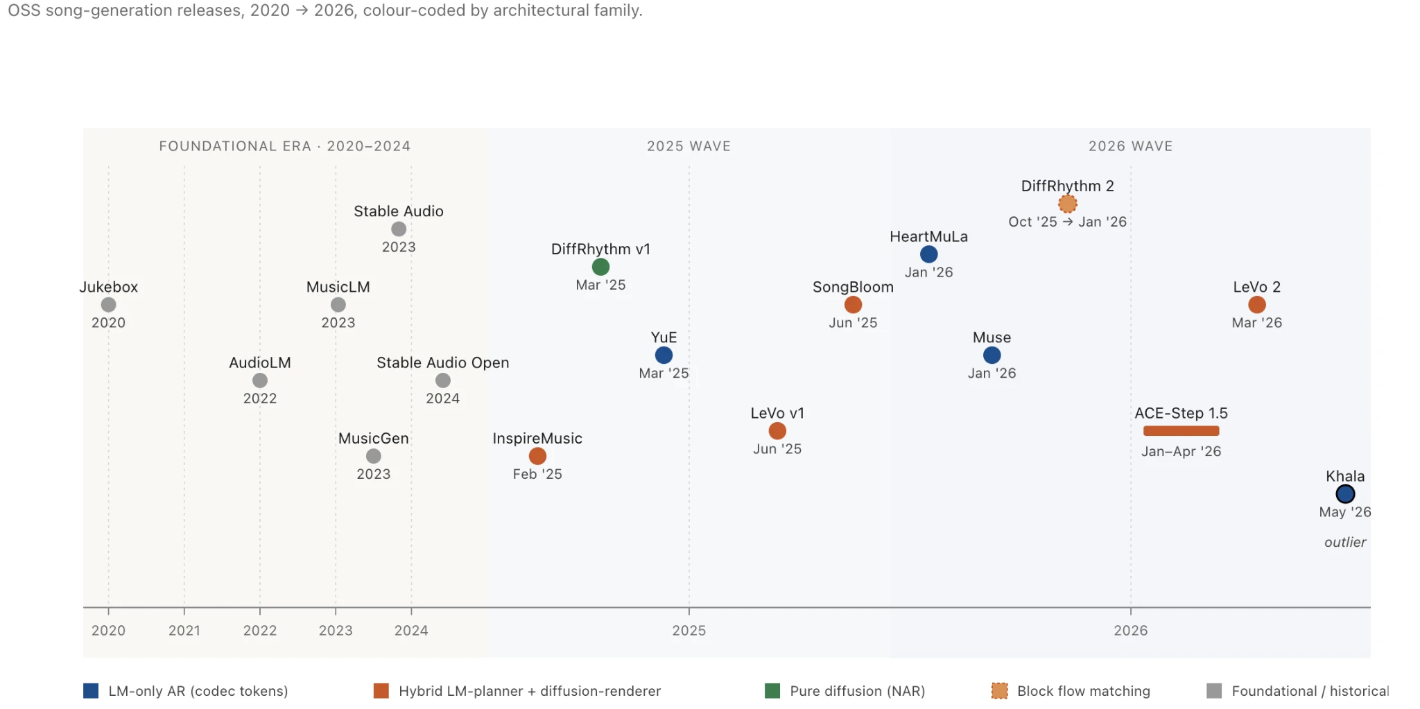
Things begin in 2020 with Jukebox (OpenAI), which set the basic recipe that subsequent open-weight music generation would either iterate on or deliberately depart from: hierarchical audio tokens, coarse-to-fine VQ-VAE, an autoregressive prior on top, lyrics conditioned through the AR backbone 🔗. Jukebox was big, slow, and impractical, but it established the engineering substrate the field has been polishing for six years.
AudioLM (Google, 2022) split the problem into semantic and acoustic tokens, treating music generation as a language-modelling problem over a learned audio vocabulary for the first time 🔗. MusicLM (Google, 2023) layered MuLan text-audio embeddings over that vocabulary and produced the first convincing text-to-music samples 🔗. MusicGen (Meta, 2023) compressed the recipe into a single-stage Transformer over EnCodec tokens, and shipped trained weights you could actually download and run 🔗. Stable Audio (Stability, 2023) and Stable Audio Open (2024) brought continuous-latent diffusion into the picture and contributed a music VAE that several 2026 open-weight models still use as their audio representation 🔗. The codec lineage that matters for what comes next runs EnCodec → DAC → MuCodec / X-Codec / Stable-Audio-VAE; the choice between them affects how a model sounds more than its parameter count does.
Meta was moving in a different direction at the same time: SAM Audio targets sound separation rather than generation, using much of the same diffusion substrate.
The 2025 wave is where the open community begins shipping models a practitioner can take seriously. DiffRhythm v1 (ASLP@NPU) made fast non-autoregressive diffusion practical for full-song generation, at RTF 0.034 on an RTX 4090 (around 28× realtime), with a phoneme-G2P lyric conditioning route that required sentence-start timestamps – one of the few details that still distinguishes the DiffRhythm line from the rest of the field, since almost everyone else moved to raw text 🔗. YuE (M-A-P) was the 7B LM-only system that quantified RoPE long-range decay and used that finding to justify segment-based conditioning, a pattern every subsequent full-song generator has since adopted 🔗. InspireMusic (Alibaba FunAudioLLM) brought a Qwen2.5 LM-planner over a flow-matching renderer into the open, though only its instrumental checkpoint shipped 🔗. LeVo v1 (Tencent SongGeneration v1) introduced the multi-stage DPO pipeline that LeVo 2 inherits and extends, with three separate offline DPO runs (lyric alignment, prompt consistency, musicality) merged by linear weight interpolation 🔗. SongBloom (Tencent and CUHK-Shenzhen) interleaved autoregressive planning with diffusion refinement and required a reference audio clip at inference, which is what puts it slightly outside the text-only comparison this post runs 🔗.
The 2026 wave, in roughly chronological order. HeartMuLa (institutional affiliation undisclosed in the paper) shipped early in the year with a multi-encoder codec (Whisper plus WavLM plus MuEncoder fused into a single 12.5 Hz quantizer, the lowest frame rate in the slate) over a hierarchical Llama-3.2-based LM with factorized DPO along the global/local seam 🔗. Muse (Fudan) followed with a deliberately vanilla 0.6B Qwen3 LM over MuCodec – no diffusion, no RL, no auxiliary losses; the contribution was not the architecture but the training corpus: 7,771 hours of fully synthetic Suno-V5 output, openly licensed, the only fully released training set in the slate 🔗. ACE-Step 1.5 (ACE Studio and StepFun) added an FSQ tokenizer to the v1 hybrid stack, shipped the most aggressive remix / edit / cover tooling in the field, and remains the only model whose alignment is fully intrinsic, with the DiT-side reward computed from its own attention geometry rather than a human-preference dataset 🔗. DiffRhythm 2 (Xiaomi Research and ASLP@NPU) introduced Block Flow Matching – non-autoregressive within blocks, autoregressive across them, KV-cached at the boundary – together with Cross-Pair Preference Optimization on 40,000 pairs in roughly 200 GPU-hours 🔗. LeVo 2 (Tencent SongGeneration v2) scaled LeVo v1 to about 4 B parameters and added a semi-online DPO stage with aesthetic scoring on top of the offline DPO base 🔗; the model arrived without a paper, and the technical report has been promised but not shipped. Khala (Central Conservatory of Music) is the year’s outlier, with a 64-layer-deep RVQ over pure acoustic tokens, no semantic stage, and a Task-0 hybrid-attention training trick standing in for the semantic conditioning every other model uses 🔗. The architecture revives Jukebox’s pure-acoustic-only thesis specifically – not the broader Jukebox influence on hierarchical audio tokens and the codec lineage, which is already visible everywhere above.
Two architectural families dominate that 2026 list, and the colour-coding in Figure 1 makes the split visible at a glance. The first is LM-only autoregressive over codec tokens, in which a transformer predicts the next audio token given lyrics and conditioning – YuE, HeartMuLa, Muse, and Khala live here. The second is hybrid LM-planner plus diffusion-renderer, in which an LM plans structure and a separate diffusion model renders frames – ACE-Step 1.5 and LeVo 2 live here. DiffRhythm 2’s Block Flow Matching belongs to neither cleanly; it is non-autoregressive within blocks and autoregressive across them, which makes it a hybrid by a different route. DiffRhythm v1 is the only remaining inhabitant of a third family that 2026 has otherwise left behind, pure non-autoregressive diffusion. The trade-offs each family makes – alignment cleanness, inference speed, audio fidelity, tooling reach – are what §3 walks through.
Which open-source model wins? A deep dive into each contender
We walk the slate in two passes. First, the three models that warrant a real deep-dive – the research substrate, the audio-quality winner, and the architectural outlier. Then six honorable mentions, each kept tight: enough to place the model and call out the one or two things that matter.
Is ACE-Step 1.5 the best open-source model for fine-tuning and remixing?
ACE-Step 1.5 is two things at once, and this section is going to walk both. It is the best target in the slate for fine-tuning, remixing, continuation, and any downstream work that benefits from a permissive license and rich tooling – by a margin large enough that there is no real second place. It is also the model whose audio carries the slate’s most distinctive artifact: a metallic shimmer we hear across the full runtime, on vocals and on instrumental sections alike. The architecture and the artifact share at least one suspect (the codec / tokenizer change between v1 and 1.5), which is why the model warrants a deep-dive rather than a one-line dismissal of either half.
Architecture. ACE-Step 1.5 is a hybrid LM-planner plus diffusion-renderer. A Qwen3-based LM sits upstream and produces a structured plan – BPM, key, duration, structure tags, lyric placement – and a DiT (around 2 B parameters in the standard variant, 4 B in 1.5 XL) renders audio frames given the plan 🔗. The audio representation pairs a custom 1-D VAE (Muon-trained) with an FSQ tokenizer operating at 5 Hz – among the lowest frame rates in the slate, in the same bracket as DiffRhythm 2 – and decodes to 48 kHz stereo. The MIT license covers both code and weights, and the HuggingFace model card carries a verbatim grant – “You can strictly use the generated music for commercial purposes” – that is unusually explicit for this field 🔗. We will return to the codec choice at the end of the section, because the tokenizer at 5 Hz is the load-bearing variable in our working hypothesis about the artifact.
The showpiece – intrinsic RL. This is where ACE-Step 1.5 does something nobody else in the 2026 slate does. Every other model that uses preference optimization (LeVo 2, HeartMuLa, DiffRhythm 2) needs preference data – pairs of (winner, loser) clips, labelled either by humans or by an external metric. ACE-Step 1.5 does not. Its reward signal comes from the model’s own internal state.
The intuition first, because the formal mechanism takes a paragraph to unpack. A DiT generating audio from lyrics learns a cross-attention map between the lyric tokens and the audio frames. If the model is doing its job, the map looks roughly like a diagonal stripe – lyric token n attends to audio frame m, with m increasing monotonically as n does. When the model goes wrong, the stripe goes wrong: it skips lyric tokens (gap), wanders backwards (singer goes out of order), or smears across many frames (alignment too fuzzy). ACE-Step’s training loop reads those properties off the attention map directly and turns them into a scalar reward.
The mechanism is called the Attention Alignment Score (AAS) 🔗. It computes both directions of the attention map (lyric-to-audio and audio-to-lyric, so direction-consensus matters), then aggregates three sub-scores by Dynamic Time Warping: Coverage (did the singer sing every word?), Monotonicity (did the singer sing them in order?), and Path Confidence (how sharp is the alignment stripe?). The paper claims AAS correlates above 95% with human lyric-audio-sync judgements – a number we hold lightly because there is no before-and-after-RL PER ablation accompanying the claim, but the recipe is internally coherent. AAS feeds into a DiffusionNTF training loop, where DiffusionNTF is RL on diffusion via the forward noising process, which sidesteps the slow reverse-sampling-chain gradients that usually make RL on diffusion expensive 🔗. The LM side is GRPO with a Pointwise Mutual Information reward between generated captions and generated audio codes 🔗. Final LM reward weighting is 50% stylistic atmosphere, 30% lyric content, 20% metadata.
ACE-Step 1.5 is the only model in the slate whose alignment reward is defined by its own attention geometry. No human preference dataset, no external reward model, no third-party metric being optimized. RLHF without the H – reward from internal consistency, not from a downstream signal. The picture is unusual enough that, taken on its own, the paper would be a notable contribution to the alignment literature.
Omni-Task, because the foundation-model framing materializes here. The same DiT weights run six task modes via two knobs – what to condition on (Source Latent) and which output regions to overwrite (Mask) 🔗. The modes are text-to-music (synthesize from scratch), cover (re-synthesize timbre over an existing melodic skeleton), repainting (regenerate a time-window inside a track), track extraction (a generative stem separator), layering (add complementary instruments to an existing track), and completion (orchestrate a full arrangement from a single motif). No other 2026 model in the slate runs editing modes out of a single set of weights. The LM has four complementary modes – Planner (free text → structured YAML), Listener (audio → captions and lyrics, which is what makes the PMI reward possible), Co-Pilot (sparse query → full song structure), and Refiner (raw user input → canonical conditioning format) 🔗. Whether all four are exposed as user-facing endpoints or live inside the inference loop is not clear from the paper alone, but the framing is plain: ACE-Step 1.5 is positioned as a substrate, not a song-in-song-out service. That positioning is what makes it the research and fine-tune winner even though it is not the audio-quality winner.
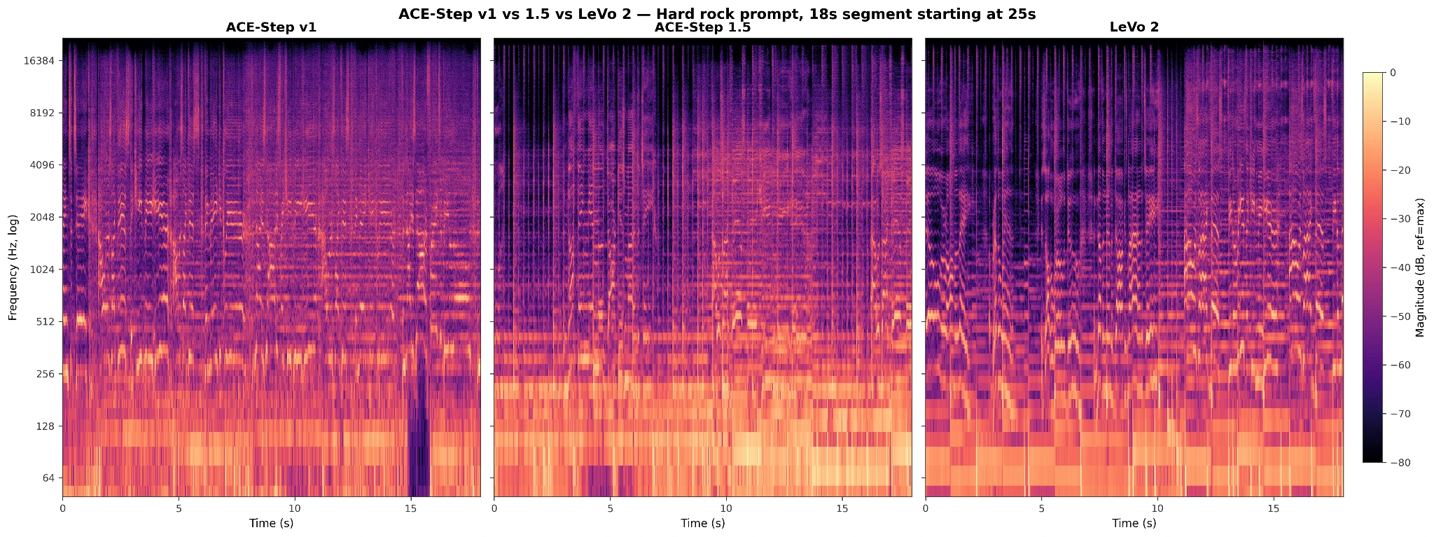
The audio verdict. ACE-Step 1.5 has a recurring metallic shimmer that we hear on sustained vowels and on cymbal-heavy instrumental passages alike. The cleanest place to hear it is the chorus of the Hard-rock sample around the second held “unknown” – the vowel tail goes glassy in a way nothing else in the slate does on the same prompt. Crucially, the artifact persists into the instrumental sections, which rules out the most obvious explanation (a vocal-codec-specific compression artifact). Our working hypothesis is that the artifact comes from either the DiT denoiser at low step counts or the FSQ tokenizer at 5 Hz – both are the components that changed between ACE-Step v1 and 1.5. We hold the hypothesis lightly: we have not done the obvious ablations (rerun the 1.5 weights with more diffusion steps, swap the FSQ stage), and we are working from listening, not from a controlled internal probe. What we do have is one piece of internal evidence pointing the same way: ACE-Step v1, which uses a different codec and tokenizer, does not have these artifacts. v1 trades that cleanness for weaker musicality. Figure 2 puts ACE-Step v1, ACE-Step 1.5, and LeVo 2 side by side on the same prompt; the spectrogram does not isolate the metallic character of 1.5 on its own, but the comparison to LeVo 2’s upper-band cleanness lines up with what the audio says.
If your work is fine-tuning, LoRA-training, downstream tooling, remixing existing tracks, or any pipeline that needs to extend the model rather than only call it, ACE-Step 1.5 is the right model in the slate. If you need pristine audio for end-user playback right now, the artifact will bother you, and the next deep-dive is the model you should keep reading for.
LeVo 2 review: does it produce the most natural-sounding AI music?
LeVo 2 is the quality winner of the slate, and the cost is the license. Across the three style-and-lyric combinations we tested, LeVo 2 produced the most organic and most natural-sounding clips of any model in the comparison; the verdict held on hard rock, on jazz, and on pop, and it is not the kind of verdict that depended on seed luck. The catch is that LeVo 2 ships under a Tencent custom license that forbids any commercial or production use, and that license arrives wrapped in some documentation noise we will untangle in a moment.
A note on documentation, because it shapes everything below. LeVo 2 is the only model in our slate without a standalone arXiv paper. The canonical documentation is the GitHub README, supplemented by the v1 paper for everything architectural that v2 inherits, plus a “technical report” that has been promised since 2026-03-01 and as of this writing has not shipped 🔗. Every load-bearing claim about LeVo 2 in this section carries the same caveat: vendor-self-reported, README-only, no third-party reproduction yet.
Architecture. LeVo 2 is a hybrid LM-planner plus diffusion-renderer, in the same family as ACE-Step 1.5 but from a different lineage. The LeLM transformer plans structure and lyric placement; a Music Codec DiT denoiser renders audio frames given the plan 🔗. v2 scales the LeLM to roughly 4 B parameters (from v1’s 2.136 B), though whether the 4 B refers to the LeLM alone or to LeLM plus the carried-over codec is not clarified in the README. Three inference VRAM tiers are documented for the first time in the LeVo line (10 / 22 / 28 GB), and maximum song length is 4 min 30 s.
License, verbatim – and the HuggingFace card is wrong. The Tencent custom license covers both v1 and v2 via a single LICENSE file on the main branch 🔗. The load-bearing clause: “You agree to use the SongGeneration only for academic, research and education purposes, and refrain from using it for any commercial or production purposes under any circumstances.” The grant explicitly excludes training data and “other AI components” from its scope, so reward models, annotation pipelines, and the aesthetic-scoring framework discussed below are not covered either. The HuggingFace model card for v2-large reads `— license: unknown —` because the weights are hosted on an individual account (`lglg666/SongGeneration-v2-large`) rather than under the Tencent organization 🔗. That is misleading at best; the actual license is the Tencent custom non-commercial described above, and anyone considering building on this model should read the LICENSE file, not the HF card.
The showpiece – the alignment pipeline. The reason LeVo 2 sounds the way it does is, almost certainly, the most aggressive preference-optimization pipeline of any model in the slate. LeVo v1 introduced multi-strategy offline DPO: three independent DPO runs along three preference axes (lyric alignment via ASR phoneme-error gap, prompt consistency via MuQ-MuLan similarity, musicality via a reward model trained on ~4,000 crowdsourced ranking seeds), and the three resulting fine-tunes were merged by linear weight interpolation 🔗. The merge is the part worth noticing. Mixing the three preference datasets into one training run loses on most metrics – the gradient gets pulled in contradictory directions, because lyric alignment and musicality genuinely trade against each other. Training three separate models and combining them in weight space sidesteps that. The interpolation coefficient is exposed as a knob.
LeVo 2 keeps that base and adds a semi-online DPO stage with aesthetic scoring on top 🔗. “Semi-online” is the new term and worth defining: standard DPO is offline – preference pairs are collected once and the policy never generates fresh candidates during training. Online DPO refreshes pairs every step, sampling fresh candidates from the current policy and scoring them on the fly (closer to PPO-style RLHF in cost). Semi-online sits between the two: the policy generates fresh candidates periodically, gets them scored, and refreshes the preference set, so the pairs reflect the current model’s distribution without paying for fully online sampling. The reward model used in this stage is not specified in the README; the most plausible candidate is the “Automated Music Aesthetic Evaluation Framework” that the same README lists as a TODO release, which would make the reward model a Tencent-team artifact, echoing the same-team-metric pattern v1 had with MuQ-MuLan.
The pipeline size moved with the strategy. v1 used roughly 60,000 preference pairs total across three axes; v2 reportedly uses about 200,000 pairs through the offline stage plus the periodic refresh in the semi-online stage. v2 reports PER 8.55% against Suno V5’s 12.4% on an undisclosed test set with an undisclosed ASR – a comparison we will not endorse without disclosure, but the broader point holds: LeVo 2 has had more, and more sophisticated, preference optimization applied to it than any other model we tested. That is plausibly why it sounds the way it does.
The audio verdict. LeVo 2’s clips sit in the mix the way recorded music does. The vocals avoid the metallic register that ACE-Step 1.5 falls into; the timbre work is plausible enough that on the jazz prompt it is not hard to forget for a few seconds that the take is synthetic; arrangements feel arranged, not interpolated. We do not have an ablation that isolates which part of the alignment pipeline did which work, but the pattern is consistent enough that we will say it plainly: among the eight models in our experiments, LeVo 2 is the one whose output we would most confidently call music rather than a generated audio file. The price of that verdict is the license. If you can live inside academic, research, or education use, LeVo 2 is the model to use. If you cannot, the verdict still stands, but the model that wins on quality is not the model you can ship.
What makes Khala the most architecturally unusual model in the 2026 slate?
Disclaimer the authors pinned to the repository as of May 2026:
We have identified a potential issue that may significantly affect inference quality. The problem is currently under investigation and may be related to numerical precision. Until this notice is removed, please treat current generation quality as unstable.
Khala is the most architecturally distinctive thing the 2026 wave produced, and the audio – even under the disclaimer – is doing something none of the other models do. In some cells, the model produces melodies and vocal motifs that nothing else in our slate produces; in others, the audio comes out structurally simple in a way that pulls the listening verdict back toward the disclaimer. The architecture is interesting enough that the deep-dive is worth writing under provisional listening, and we will revisit the verdict if the fixed release changes the picture.
Khala is the only 2026 model that revives Jukebox’s pure-acoustic, no-semantic-stage thesis 🔗. The precision matters because Jukebox’s broader influence – hierarchical audio tokens, coarse-to-fine RVQ-style coding, the whole EnCodec → DAC → MuCodec lineage that runs through the field – is felt across every model in the slate, including the ones that are otherwise nothing like Jukebox. What Khala specifically revives is the part that consensus walked away from: doing music generation in acoustic-token space only, with no semantic-token stage between the lyrics and the audio frames. Every other model we tested (YuE, HeartMuLa, Muse, ACE-Step 1.5, LeVo 2, DiffRhythm 2) uses semantic tokens, a diffusion-based renderer, or both, on the assumption that pure acoustic-token autoregression hit a ceiling at the Jukebox scale for reasons that should not be re-litigated. Khala bets those reasons were wrong, or at least worth retesting now that codecs and compute have moved on by six years.
Architecture. Three networks in series, with a total parameter budget that lands mid-pack for the slate. A 1.6 B-parameter backbone autoregresses over the coarsest RVQ layer – the layer carrying most of the structural information. A 1.8 B-parameter super-resolution stage fills in the finer RVQ layers above the coarse one. A 0.27 B-parameter codec handles the encode-and-decode round-trip 🔗. Total: roughly 3.7 B parameters across the three. The interesting number is the codec depth – Khala runs a 64-layer-deep RVQ, which is the deepest in our slate by a substantial margin. Deep RVQ buys reconstruction fidelity at the cost of longer token sequences to predict, and the bet behind 64 layers is that the depth lets the autoregressive backbone work in pure acoustic space without needing a separate semantic abstraction to hold the structure together.
The mechanism standing in for the semantic stage everyone else uses is Task-0 hybrid attention 🔗. During training, the model runs two attention modes side by side: causal attention for a Task-0 lyric-alignment objective (the model has to predict lyric tokens in time-aligned position alongside audio tokens), and full attention for layer-wise audio refinement. At inference, Task-0 is not used; it is a training-time architectural induction, not a separate forward pass. The framing in the paper is that this lets text-and-vocal alignment emerge without an explicit semantic bridge, the way that bridge would exist in a model running a HuBERT or W2V-BERT semantic stage between lyrics and audio. Whether the trick actually compensates for the missing semantic stage is the empirical question Khala exists to answer.
The training corpus is the second distinctive piece, and worth a paragraph on its own. Khala was trained on roughly 18 million tracks comprising 1.2 million hours of audio, drawn from the Central Conservatory of Music’s internal music dataset 🔗. The hours number is the largest in our slate. The more interesting fact is that this is a different species of training data from everything else in the field – an institutional music-conservatory archive rather than scraped Internet audio. Provenance is documented at the institutional level (conservatory dataset, internal use) but not per-track; better than the “we say nothing” pattern most papers fall into, not as transparent as Muse’s fully published synthetic corpus. The contribution worth flagging on its own terms: conservatory archives are a different bucket of training data, with a different stylistic distribution, a different acoustic provenance, and a different legal posture from the audio scrapes everyone else trains on. Seeing a 1.2 M-hour model trained from one is unusual, and we are interested in what training on archive-grade audio specifically buys.
License. Khala ships under CC BY-NC 4.0 – non-commercial like LeVo 2, but for different reasons (conservatory data provenance and institutional norms rather than corporate IP).
The audio verdict, under the disclaimer. Khala has a noticeable AI character that we hear in the arrangements first. Many of the generations come out structurally simple, light on harmonic motion, light on the rhythmic risk-taking that gives generated music a sense of personality. The model is also genuinely unstable run to run, and the intros are often messy in a way none of the other models in the slate are – the first few bars take time to find their footing, which is consistent with the failure mode the authors are warning about. Vocals are not consistently expressive across cells; some are flat in a way that reads as obvious model-output. A few generations also have natural-sounding voices that compare favourably to the deep-dive winners. LeVo 2 still wins aggregate audio quality across the cells we have, but Khala is not a model to dismiss: the bet on deep-RVQ pure-acoustic autoregression is producing genuinely different output on some prompts, and the disclaimer suggests the current state of the model is not its ceiling. The messy intros and run-to-run instability read as likely to improve with future code updates, which is also what the disclaimer is pointing at.
To close, Khala is the architectural outlier of the 2026 slate: a different bet from everyone else, with audio that supports the case on some cells and undermines it on others, and with the disclaimer still attached. The license keeps it out of commercial product work alongside LeVo 2. For research, for understanding where the field could still go, and for anyone interested in routes through music generation that the consensus has closed prematurely, Khala is the model to pay attention to over the next six months.
How do YuE, HeartMuLa, Muse, and DiffRhythm 2 compare?
YuE (M-A-P, Apache 2.0) is the 2025 lineage anchor of the 2026 wave and the place to start a careful honorable-mentions read 🔗. Its paper did something rare in this field – it quantified the failure mode it was solving. The claim that “degradation begins around 3K tokens, complete failure beyond 6K tokens” without chain-of-thought conditioning is what justifies the segment-based conditioning recipe (~14 sections per song, ~30 s each, with text plus lyrics plus audio interleaved per section) that every post-YuE full-song generator has since adopted. The paper also includes a Limitations section that names its own failure modes, which is the kind of behaviour we would like to see more of in the field. The license is Apache 2.0 with an explicit commercial-use grant.
The listening verdict is less generous than the lineage credit. YuE’s audio did not stand out on quality or musicality across the three styles we ran; the more practical drawback is inference speed. On an RTX 4090, YuE runs at roughly 12× slower than realtime, which makes running a small experimental sweep a noticeable time cost – and over a long enough horizon, time cost is itself a quality cost, because it bounds how much prompt iteration you can afford. Community forks (YuEGP, YuE-exllamav2) exist precisely because of this.
HeartMuLa
HeartMuLa (Apache 2.0 code) is the slate’s interesting-codec model with a less-interesting audio verdict 🔗. The novel contribution is the codec design: HeartCodec runs at 12.5 Hz – the lowest frame rate in the slate – and fuses three encoders (Whisper plus WavLM plus MuEncoder) into a single quantizer. Most music codecs use one encoder; HeartCodec’s bet is that mixing semantic-leaning encoders with an acoustic one yields a richer token distribution. The LM on top is Llama-3.2 in a hierarchical Global plus Local configuration, with DPO factorized along the global / local seam – clever paper-craft, empirical lift over a monolithic DPO baseline left unmeasured.
Our listening verdict: HeartMuLa sounds the same across styles. We tried hard rock, jazz, and pop, and what came back was generic pop in every case – averaged, smoothed, AI-blurry. We frame this carefully, because it could be a weights or inference quirk on our end, but the consistency across all three prompts pushes the explanation toward something structural in the released checkpoint. One small note for the careful reader: HeartMuLa’s abstract claims significant gains at 7 B parameters, but only 3 B SKUs ship.
Muse
Muse (Fudan, MIT code, Apache-2.0 weights, MIT data) is in the slate for one reason that has nothing to do with its architecture and everything to do with its training data 🔗. The model itself is deliberately vanilla – a 0.6 B-parameter Qwen3 over MuCodec, single-stage SFT, no diffusion, no RL, no auxiliary losses. The paper says this in so many words: “without task-specific losses, auxiliary objectives, or additional architectural components.” The bet is not on the model; the bet is on the corpus: 7,771 hours of fully synthetic Suno-V5 output, generated by Suno V5 plus GPT-5-mini plus Qwen3-Omni-30B, released MIT, the only fully released training corpus in the slate. If you want to train a competitor on the same data, you can. That is the contribution.
The headline claim – that 0.6 B Muse beats 8 B YuE on every column of a SongEval benchmark – does not survive a careful reading: the test set is 100 songs, there are no confidence intervals, and SongEval is published by a different team that is itself a competitor (DiffRhythm). We will not endorse the “beats YuE” framing. What our own listening said is more modest: Muse’s general audio quality is better than ACE-Step 1.5 in the cells we ran, and the model produces audio with a distinct Chinese-leaning “accent” on English-prompt vocals – most plausibly because the synthetic corpus was Chinese-curated even though Suno V5 was the synthesis engine. The legal hinge worth flagging: Muse’s openness rests on Suno’s terms of service permitting this kind of derivative use, and the paper does not engage that question.
DiffRhythm 2
DiffRhythm 2 (Xiaomi Research and ASLP@NPU, Apache 2.0) is the architecturally most novel thing in the 2026 slate, and also the slate’s most paper-honest model 🔗. The architecture is Block Flow Matching: split the latent into blocks of about two seconds, denoise within each block in parallel (the non-autoregressive part), and condition each block on all previous clean blocks via KV-cached attention (the autoregressive part). The result is semi-autoregressive – fast within a block, structured across blocks, with KV caching at the block boundary keeping inference cheap. The alignment recipe is Cross-Pair Preference Optimization on 40,000 pairs in roughly 200 GPU-hours total, which is strikingly small for an open-source state-of-the-art claim (the GPU type is not named).
The audio verdict has two halves. On the positive side, DiffRhythm 2 has the lightest style-impact across genres of anything in our slate – different style prompts genuinely produced perceptibly different-feeling generations, which is harder than it sounds and several models in this list fail at. On the negative side, the audio is more artificial than the deep-dive winners, the rhythm is genuinely unstable (which is a quietly funny finding given the model is named DiffRhythm), and the paper itself flags vocal quality as behind ACE-Step and LeVo in §5.2. One possible cause of the rhythm instability that we offer as a hypothesis rather than a finding: DiffRhythm 2 is among the few models still using phoneme-based lyric conditioning, and phonemes strip prosodic and timing cues that raw-text models retain. The most useful thing we can say about DiffRhythm 2 is that its paper says what is wrong with it without our needing to ask: §6 contains the “Open-source still falls short of commercial systems overall” line that the rest of our post borrows as a thesis quote, and §5.2 admits the vocal-quality gap to ACE-Step and LeVo directly. Vendor-side honesty of this kind is rare, and it earns the model the credit we are giving it here.
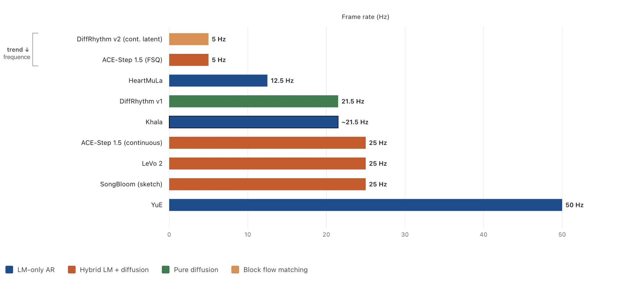
Frames per second of the audio representation each model’s LM (or diffusion) operates on. Some are discrete codec tokens; others are continuous VAE latents — the relevant axis is the same.
How do you evaluate AI-generated music quality?
Song generation is harder to evaluate than text-to-speech, and nobody has settled on what good evaluation looks like yet. Our own pass is small: three style-and-lyric prompts at one seed per model, what a practitioner with a cheap GPU and a week to listen would actually manage. Not a benchmark. A practitioner’s pass.
A text-to-speech system can be scored by intelligibility, which is roughly a scalar: did the listener understand the words? A song-generation system has to be scored on intelligibility and on musicality, mix balance, emotional fit, style adherence, structural coherence, vocals creativity, and how the vocals sit against the instrumental. Most of these resist single-scalar measurement, and many of them interact – a vocal that is more intelligible may be less expressive, a mix that is cleaner may be flatter, an arrangement that adheres more tightly to the prompt may be more boring. There is no current benchmark that captures the whole picture cleanly, and the ones that try are doing real work by trying.
The WER caveat that almost every paper buries. Almost every paper in this space reports a Word Error Rate or a Phoneme Error Rate as a load-bearing intelligibility metric. WER and PER are computed by running an ASR over the model’s outputs and comparing the transcript to the lyric input. The catch – and the reason careful readers should treat WER as a soft signal – is that the ASR is itself a model with its own failure patterns. A model that produces audio the ASR happens to like will get a better WER than a model that produces audio the ASR happens to find unfamiliar, regardless of how intelligible the audio is to humans. We have heard cases where a model with a better-reported WER is subjectively less intelligible to a human listener than a model with worse-reported WER. The right reader habit is to ask which ASR was used and how it was chosen.
Subjective surveys are still the best signal, and consistently underpowered. The single most useful thing a paper can do is run a properly powered subjective evaluation: enough raters, blind to model identity, with explicit rating dimensions, scored across enough samples that fatigue does not dominate the result. Most papers in this space ship subjective evals with 9 to 40 raters per metric, which is enough to spot a large effect and not enough to distinguish close calls. LeVo v1 used 10 paid professionals across 20 lyrics × 3 modes. HeartMuLa used 9 raters across 20 samples. YuE used about 40 evaluators with an unexplained split. DiffRhythm v1 used 30 listeners. DiffRhythm 2 used 10 pro listeners. Muse used zero humans – all of its headline metrics are automatic. These are not bad numbers for the constraints, but anyone reading the resulting tables should know what those constraints are.
SongEval, SongBench. Two benchmark efforts in this space deserve real credit. SongEval (published by the DiffRhythm team at ASLP@NPU) is the closest thing the field has to a shared subjective-evaluation framework, and several 2026 papers report numbers on it as a load-bearing metric: ACE-Step §5.1, DiffRhythm 2 §5.1, HeartMuLa Tables 7–11, Muse §5.3. SongBench plays a similar role for parts of the slate. Building benchmarks is mostly thankless work; the only reason the model teams are also the benchmark teams is that nobody else is doing it.
Four of the eleven Tier-A 2026 models report SongEval numbers, and SongEval comes from one of those eleven teams. MuQ-MuLan, which LeVo uses as a headline text-audio similarity metric, is a Tencent same-lab artifact. HeartMuLa’s PER pipeline uses HeartTranscriptor, which is HeartMuLa’s own ASR – the same ASR is used to compute (a) HeartCodec’s WER table, (b) HeartMuLa’s PER table against competitors, and (c) the reward signal for one of three of its DPO sets. None of these patterns mean the numbers are wrong. They mean that reading those numbers should include the question of who built the metric, alongside the question of what it measures.
Benchmark tables are one half of the evaluation problem. The other half is knowing what those benchmarks are measuring on, and that question hits a wall almost immediately.
Of the eight models in our slate, exactly one (Muse) releases its training corpus.
Every other paper either omits training data entirely, names it only at an institutional level (Khala’s “internal music dataset”), or acknowledges internet-sourced material whose provenance no one can audit.
The field’s training-data opacity is its most structural problem, and no single model team can fix it. No one is obliged to. But anyone running a comparison is implicitly trusting eight different opaque pipelines, and that trust has no verifiable floor.
One clean direction toward solving this is licensed synthetic data: training corpora generated by other models whose outputs the trainer has clear legal rights to use, with documented generation pipelines and released datasets. Muse demonstrates the basic shape – generate audio with Suno V5, lyrics and prompts with GPT-5-mini, refinement with Qwen3-Omni-30B, release everything MIT.
Open-source music generation models compared: full listening results
Prompts
| Hard rock | Jazz | Pop |
|---|---|---|
Hard rock anthem. Male lead vocal with grit and edge — rough but melodic, not screamed. Distorted electric guitars: palm-muted single-note riffing in verses, full power chords in choruses. Driving bass, energetic 4/4 drums around 140 BPM, cymbal crashes on chorus downbeats. Anthemic shout-along chorus. Brief guitar lead between sections.
Show lyrics[Verse 1] The streetlights bow their heads to let me through The sky has spilled its silver on the lake A breath of wind is all the world will do And nothing in the dark is mine to take [Pre-Chorus] Hours like this, they keep me here Hours like this, they make it clear [Chorus] The night is not afraid to be alone The night is not afraid to be unknown And every quiet thing I cannot say Is somewhere in the way the stars are sown [Verse 2] A window glows above an empty street A radio is humming through the wall The world has slowed enough that I can meet The smaller part of me beneath it all [Pre-Chorus] Hours like this, they keep me here Hours like this, they make it clear [Chorus] The night is not afraid to be alone The night is not afraid to be unknown And every quiet thing I cannot say Is somewhere in the way the stars are sown [Bridge] And nothing has to happen for it to be enough Nothing has to ask, nothing has to hush Just the slow way midnight breathes in time With a soft and sleeping town [Chorus] The night is not afraid to be alone The night is not afraid to be unknown |
Smooth jazz quartet. Intimate male crooner vocal — warm, conversational, slightly behind the beat. Walking upright bass, brushed drum kit, warm Rhodes electric piano comping, muted trumpet fills between vocal phrases. Moderate swing, around 95 BPM. Late-night club atmosphere. Tasteful reverb, no compression sheen.
Show lyrics[Verse 1] Don't search the lines for any hidden truth These words were written purely as a test No subtle code, no clever reverse-proof Just syllables to hear if it sings best [Pre-Chorus] So close your notebook, set the verdict aside Just listen, listen, listen for the ride [Chorus] There is no message, just a melody Don't read between the lines you hear The soul of song is sound, you must agree Let go the meaning, let the music make it clear [Verse 2] A poet would be jealous, I'm aware But poetry is not what we are after We're checking if the model holds the air And if the chorus gives a little laughter [Pre-Chorus] So close your notebook, set the verdict aside Just listen, listen, listen for the ride [Chorus] There is no message, just a melody Don't read between the lines you hear The soul of song is sound, you must agree Let go the meaning, let the music make it clear [Bridge] The lyrics here are scaffolding For voices we are testing in the dark Don't take them home, don't take them anything Just check the pitch, the timbre, and the spark [Chorus] There is no message, just a melody Don't read between the lines you hear The soul of song is sound, you must agree Let go the meaning, let the music make it clear |
Modern pop ballad. Female lead vocal — breathy delivery in verses, controlled belt in the chorus. Mid-tempo, around 100 BPM, 4/4 time. Layered synth pads, crisp 808 kick with finger-snap percussion, clean electric guitar arpeggios, airy reverb tail, polished radio-ready mix. Melancholic verses lifting into uplifting chorus. Subtle vocal harmonies in the chorus.
Show lyrics[Verse 1] We taught the silence how to sing Fed it words and watched them turn to light Every echo learns a different thing Stories that the wires hold tight [Pre-Chorus] Now the static finds a melody Now the data finds a rhyme [Chorus] Hear the future humming low Through the wires, soft and slow Voices we did not compose Sing us back to who we know [Verse 2] A thousand models reaching for a tune Some get lost and some come dancing through Half a moonbeam, half a chip-design Half the heart is yours, the rest is mine [Pre-Chorus] Now the static finds a melody Now the data finds a rhyme [Chorus] Hear the future humming low Through the wires, soft and slow Voices we did not compose Sing us back to who we know [Bridge] Maybe music never needed hands Maybe it was waiting in the strands Patient as a dream Patient as a flame [Chorus] Hear the future humming low Through the wires, soft and slow Voices we did not compose Sing us back to who we know |
The listening table
| Model | Hard rock | Jazz | Pop | License |
|---|---|---|---|---|
| LeVo 2 | Tencent (non-commercial) | |||
| ACE-Step 1.5 | MIT | |||
| ACE-Step v1 | Apache 2.0 | |||
| Khala | CC BY-NC 4.0 | |||
| DiffRhythm 2 | Apache 2.0 | |||
| Muse | MIT code / Apache 2.0 weights / MIT data | |||
| HeartMuLa | Apache 2.0 | |||
| YuE | Apache 2.0 |
Which model should you use? The verdict
LeVo 2 wins on audio quality.
The verdict held across all three style-and-lyric combinations: hard rock, jazz, pop. The clips are the most natural-sounding clips of any model in our slate, by a margin that does not require a careful listening pass to detect. The cost is the Tencent custom non-commercial license, which forbids any commercial or production use. If you can live inside academic, research, or education use, LeVo 2 is the model you should use; if you cannot, the verdict still stands but the model you use is going to be a compromise.
ACE-Step 1.5 wins on research, fine-tuning, and downstream tooling.
The MIT license on code and weights, the Omni-Task editing modes, the documented architecture, and the maturing community ecosystem make it the substrate of choice for anyone building beyond a single model call. The cost is the metallic shimmer artifact we discussed in the deep-dive – audible on vocals, audible on instrumental, persistent enough across runs that it is structural rather than accidental.
Khala is the architectural outlier worth listening to.
A different bet from everyone else in the slate (pure-acoustic, no semantic stage, 64-layer-deep RVQ) producing audio that is sometimes genuinely interesting and sometimes structurally simple, all under an active stability disclaimer. The cost is two-part: the disclaimer says the current state is unstable, and the CC BY-NC 4.0 license keeps the model out of commercial work alongside LeVo 2.
Any verdict in this section will age. Some of these models are improving in real time – Khala in particular is mid-stabilization as we write, and a fixed release could reshuffle parts of the table – and the headline next-release cycle will not slow down.
Will open-source models ever close the gap to Suno?
Between 2024 and 2026, the open community built something that did not exist before: a set of models where a careful listener can occasionally mistake the output for a real recording. That happened faster than most of the field expected. The gap to Suno has not closed.
Two things keep it open, and neither is close to resolved. Training data is the harder one: the volume of music that carries a license permitting neural-network training is small, and that is not changing at any speed. The research community knows this and is working in the direction it can: leaner architectures, tighter pipelines, more from smaller corpora. Compute is real too; training any of these models from scratch sits at a cost that limits who can do it. Both constraints point the same direction: clean corpora used well, not large ones used opaquely.
We do not expect open weights to close the Suno gap cleanly. What we expect is steady architectural improvement. The shift that matters more long-term is open architectures that teams can train on data they actually own, not open weights trained on data no one else can audit or replicate. That is a different kind of open, and probably the more useful one.
IT-JIM builds music and audio AI for products: pipelines, fine-tuned models, plugin integrations. Song generation is useful well beyond end-to-end generation; it is also the foundation for editing tools and creative interfaces that no vendor API will expose. If you are deciding whether one of these models belongs in something you are building, and the evaluation in this post is not deep enough for that decision, that is the kind of work we do.