How Does Singing Voice Conversion Work? The Seed-VC Baseline
Have you ever tried singing? What about extreme rock vocal techniques, like hoarse vocals? What about doing it the same way across time? This singing technique is not as easy as it seems and requires consistent skills especially if you do it long-term. Sometimes the voice changes but the singing style should remain the same.<table
Vocal consistency across long recording sessions sits at the heart of what the music technology industry is bringing to AI teams right now.
For a broader look at how AI tools are reshaping the musician’s creative process, our AI for Musicians guide covers the spectrum, from production-workflow tools to open-source voice conversion models.
We trained a voice conversion model for this purpose. The goal: convert a specific speaker’s clean vocals into the same speaker’s distressed, hoarse delivery. Seed-VC is a strong fit for this kind of AI voice conversion: it performs well in zero-shot setups and provides a reliable starting point for fine-tuning.
For the task, we utilize a custom dataset of one speaker. It includes several takes per song to represent cleaner and more distressed vocals. The audio tracks were split into short (up to 20s) chunks that are processed so the silence duration is minimal.
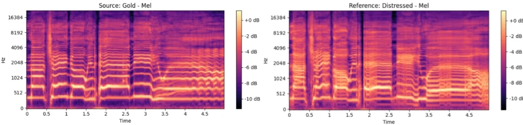
Mel spectrograms of the same segment. Gold sample is ideally clean, Distressed sample represents hoarse vocals.
The Seed-VC paper introduces two baseline flow-matching models for our task. The smaller one is designed and trained for voice conversion tasks. It extracts the source sample semantic features and target speaker style embeddings. Optionally, it uses the target mel spectrogram and semantic features for refined conversion.
The larger Seed-VC model is trained for singing voice conversion. Additionally, it has conditioning on the source fundamental frequency features to match singing vocals better. The source semantic features are aligned with the acoustic features via a length regularization module of the model.
For the task of making the singing vocals more distressed, the singing voice conversion model is a better match. We evaluated both models in a zero-shot setup on our data. The SVC model keeps the fundamental frequency of the source vocals and the conversion results sound melodically and clean. Thus, we focused on fine-tuning this model to make its result more distressed.
How Does the Seed-VC Training Pipeline Work?
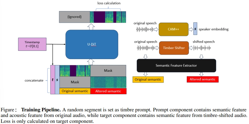
Extracted from the source utterance content features often include residual timbre information about the source speaker. To avoid the speaker timbre leakage, the Seed-VC training pipeline has an interesting modification. They use an external model as a timbre shifting model. So, during the training step, the input source waveforms are converted to simulate another speaker. The model input during training consists of the following parts:
target speaker style embeddings;
target Mel spectrogram with masked condition prompt region;
concatenated original semantic and altered semantic features aligned with acoustic features.
The loss is calculated on the masked (source) region only.
In practice, the Seed-VC training pipeline simulates a scenario where the speaker’s timbre shifts abruptly mid-segment, sometimes mid-word. The model learns to generate the full segment using the timbre captured in its opening portion.
But why do we need simulation if we can have perfectly aligned actual speaker vocals? We tried to replace the timbre shifted part of the training DiT input with the actual clean vocals and the original waveforms with the actual distressed ones.
Fine-tuning the model in these setups showed unstable loss and decrease in metrics. It made the vocals sound more hoarse but they were slightly intermittent and still not distressed enough, so we moved to the next pipeline modification.
Become More Specific About Speaker
Since we are training a speaker-specific model to change the vocal distortion, we can make the training pipeline more speaker-oriented. We can remove the prompt audio conditioning and freeze the speaker embeddings during both training and inference. We can also fine-tune the model on the distressed (reference) audio samples only.
Unfortunately, removing conditioning on the target Mel spectrogram and semantic features does not work well. It makes the conversion result louder and more noisy but does not remove the desired vocal distortion. So it still can be applied.
For freezing the speaker style embeddings, the good approach was to take the mean embeddings of the distressed vocals of the singer.
The reference-only training worked very well. It resulted in a stable decreasing trend in the loss history since now we compute loss on the full input spectrogram rather than on its small part. The vocals after fine-tuning in the reference-only setup sound much more distressed compared to the previously tried fine-tuning approaches.
Key result: Reference-only training on distressed samples produced the most stable loss curve and the most convincingly distressed output, outperforming every setup that mixed in clean vocals.
For further experimentation, we tried a couple of techniques from the YingMusic-SVC paper. This paper describes training the Seed-VC singing voice conversion model with interesting approaches.
YingMusic-SVC Fine-Tuning Approaches
Keep the Balance: Frequency-Aware Loss Balancing
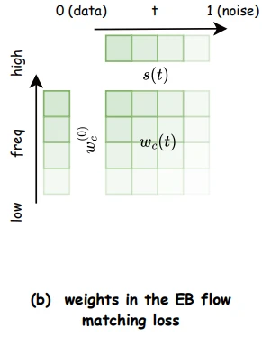
To address the imbalance in energy across frequency bands, the YingMusic-SVC paper introduces weighting coefficients for the loss function. The coefficient values increase with the frequency height and diffusion timestep. They also depend on the variance of the ground-truth diffusion velocity field.
Figure from the YingMusic-SVC paper representing the energy-balanced flow matching loss with time- and frequency-dependent weighting
Applying the loss balancing technique to our training pipeline significantly improved the fundamental frequency correlation between both the source/reference and converted audios. We tried using it with the Seed-VC native L1 loss, but it worked better when applying the L2 loss function.
Training tip: Frequency-aware loss balancing works better with L2 loss than L1. Start introducing weight coefficients from slightly lower frequencies than you might expect. The high-frequency ratio has an outsized effect on results.
The difference is audible. Below is a before/after comparison: the original clean vocal alongside the model output after reference-only training with frequency-aware loss balancing:
Before: clean vocal (Gold)
After: distressed model output
Timbre Adaptation Technique
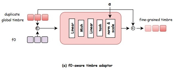
The next intriguing approach from YingMusic-SVC is designing the speaker conditioning to be time-varying and fundamental-frequency-aware. They decompose the reference singer’s representation into a static global vector and a time-varying residual that depends on the source F0 features. A small MLP network is used for this purpose.
Figure from the YingMusic-SVC paper representing the F0-aware timbre adaptor that refines global timbre embeddings into fine-grained, pitch-sensitive representations
In our experiments, using the timbre adaptor led to lower background noise in audio but decreased the fundamental frequency correlation. Combining the loss balancing strategy with the timbre adaptor helps improve the F0 metrics. So, these techniques compromise each other. But results of the model trained with loss balancing only are still better.
Style residuals cause converted samples to sound choppy: “ni-i-i-ight” instead of “niiiight”. With limited training data, the model runs out of steps to adapt the residuals before overfitting kicks in. More data is the direct fix.
Reinforcement Learning: Move Directly to the Goal?
The standout addition from YingMusic-SVC is a refining stage built on online reinforcement learning, specifically Flow-GRPO, extended with Stochastic Timestep Selection to keep noise influence more predictable. This stage runs after the regular fine-tuning phase.
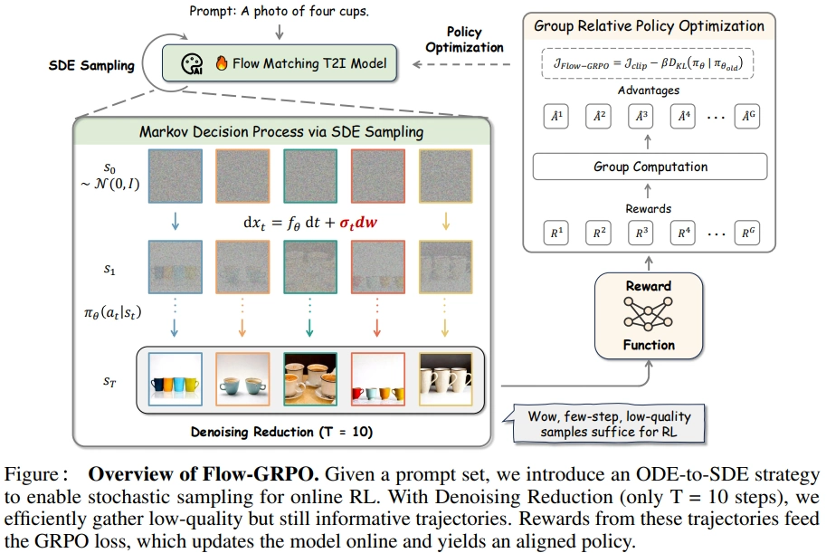
The reinforcement learning with Flow-GRPO is done in two stages. During the sampling stage, the diffusion trajectories are sampled a couple of times per prompt with noise introduction at some single step. These trajectories are evaluated with non-differentiable rewards on the final step of the trajectory. Probabilities of the diffusion timesteps are computed during the training stage. The loss function includes the perceptual reward and KL divergence loss components.
Our experiments show that Flow-GRPO raises waveform amplitude and introduces more background noise, with a drop in metric values overall. With a small dataset, a single reward outperforms a combination of several: the model responds better to one clear direction than to competing signals.
Practical note: Flow-GRPO needs a larger dataset and well-defined target metrics to deliver. With limited data, one focused reward beats a combination of several. Keep the feedback simple.
Introducing a higher coefficient for the KL divergence loss influence increases the F0 correlation between the reference and converted audio samples but this does not affect the converted audio perceptual quality.
As for any generative AI task, the main headache for our goal is the metrics. We evaluated models with DNSMOS, UTMOS and SECS scores. But these metrics do not reflect the target distortion in vocals. The target distortion results in lower DNSMOS BAK and UTMOS values. But the same does the undesired noise. Applying SECS as the reward depends on how the speaker embedding extraction model reflects the difference between the clean and distressed vocals for the same speaker.
Flow-GRPO is effective but needs a larger dataset and well-defined target metrics to deliver on its potential.
Conclusion
The singing voice conversion task is not as simple as it may seem. It requires intricate techniques, enough data amount, and irregular metric evaluation.
Our experiments show the best model performance in setup applying the loss balancing strategy for training on the reference (distressed) samples only. We simplified the model making it more speaker-specific so it does not require the reference audio samples of distressed vocals for the target speaker.
Flow-GRPO remains one of the more promising directions, but it needs more data and compute to deliver on that promise. There is always room for further experimentation. Finding the right metrics is as much part of the work as the modelling itself.
If your project involves voice conversion, singing style transfer, or any other audio AI challenge (a music product, voice cloning pipeline, or live performance tool), IT-JIM’s audio AI development team can help assess the architecture, data requirements, and path to production.
Wondering what maximum vocal distortion sounds like without a model in the loop? Here is one hour of Jimmy Barnes doing it the hard way. Consider it the upper bound.
Is there an open-source alternative to Suno in 2026?
Every couple of weeks, another open-source ai music generator model launches with a headline claiming Suno parity. Sometimes it is the abstract, sometimes a benchmark table column, sometimes a curated thread on X, but the claim is always the same: the open community has caught up. We went looking for independent head-to-head comparisons and could not find enough good material. We get asked about open-weights song generation often enough that we wanted somewhere honest to point. So we ran the comparison ourselves, on the May 2026 slate of models we could load and run.
The short answer: no, there is not an open-source Suno yet. The closest model, by our ears, gets within audible-but-real distance of Suno V5 on some prompts and trails on others; everything else trails further. DiffRhythm 2 makes the same call in its own paper: “Open-source still falls short of commercial systems overall.” 🔗. We agree. The rest of this post is the longer version of why.
There is no single open winner across all the things you might care about.
The model that produced the most natural-sounding music carries a non-commercial license.
The model best suited to research, fine-tuning, and continued experimentation is permissively licensed but has audible artifacts.
A third model in the set is the most architecturally distinctive thing released in 2026 and currently ships with a stability disclaimer from the authors themselves. Roughly: the model that wins on quality wins at a license cost, and the model that wins on freedom and tooling wins at an audio cost. Which compromise is the right one depends on what you are trying to build, and the rest of the post walks through that trade-off model by model.
Want to skip straight to the audio comparison? Jump to the listening table.
There has been a real wave of strong work in this space. The engineering behind several of the 2026 releases is substantial, and we will say so when we get to them. But the announcement layer makes that wave hard to read honestly: launch posts cherry-pick the best seeds, comparison tables come from the teams who also publish models, demo reels are curated, every release claims to be state of the art on a benchmark its own authors built. After enough cycles of this, even experienced readers stop trusting the headlines and start downloading the weights themselves, which is expensive in time. We did that work, on the cheaper kind of cloud GPU, on the same three style-and-lyric combinations across every model. The post is for the reader who would otherwise have to do it: product leads weighing whether song generation belongs in something they’re building, musicians evaluating tools, engineers choosing a base model to fine-tune, researchers trying to read the field’s current direction, anyone deciding whether to spend a weekend wiring one of these into a pipeline.
We build custom music and audio AI for products: inference pipelines, fine-tuned checkpoints, DAW plugins. The comparison below comes from the same kind of evaluation work we run for clients choosing a base model.
One honest caveat about how we tested. Each model has its own hyperparameters, its own training-data distribution, its own implicit prompt conventions. We ran three style-and-lyric combinations on each model with one seed apiece, and we are reporting what we heard from a careful pass over those clips. Longer experimentation – more prompts, fine-tuning, a real cost-quality curve – could push any of these models harder than we did. If you are deciding whether to bet on one for a real product and want a deeper investigation than fits in a blog post, that is the kind of work we do professionally at IT-JIM.
Why bother with open weights at all. The reasons are practical. Open weights let you fine-tune on your own data, build tools that vendor APIs will not expose, run offline when latency or cost or privacy require it, and ship pipelines without a per-song fee. The permissively licensed entries also let you actually ship a product on top of them. If none of those constraints apply, Suno is the easier path. But if any of them do, the model choice matters and is not currently obvious, which is what this post tries to fix.
Those are the cases we see most often in practice: teams building internal tools, labels setting up generation pipelines, plugin developers who need to run inference on-device.
Where open-weight models sit relative to commercial platforms is something we covered in our AI tools for musicians post, if that wider frame is useful before the model walk.
Which open-source music generation models did we test?
Before the timeline or the verdicts, here is the slate: eight open-weights song-generation models we tested for this post. They are
ACE-Step v1 and v1.5
LeVo 2
Khala
YuE
HeartMuLa
Muse,
DiffRhythm 2.
The timeline below mentions a fair few more – predecessors and lineage anchors that shaped the field but aren’t the right targets for a 2026 head-to-head – and from that wider set we picked the latest and most credible for the experiments. A couple we considered and then set aside (SongBloom, which requires a reference audio clip at inference, and InspireMusic, which ships only instrumental) come up later when they are relevant. If you notice something genuinely important is missing, tell us – the field moves fast, and we are happy to update.
How did open-source music AI reach where it is today?
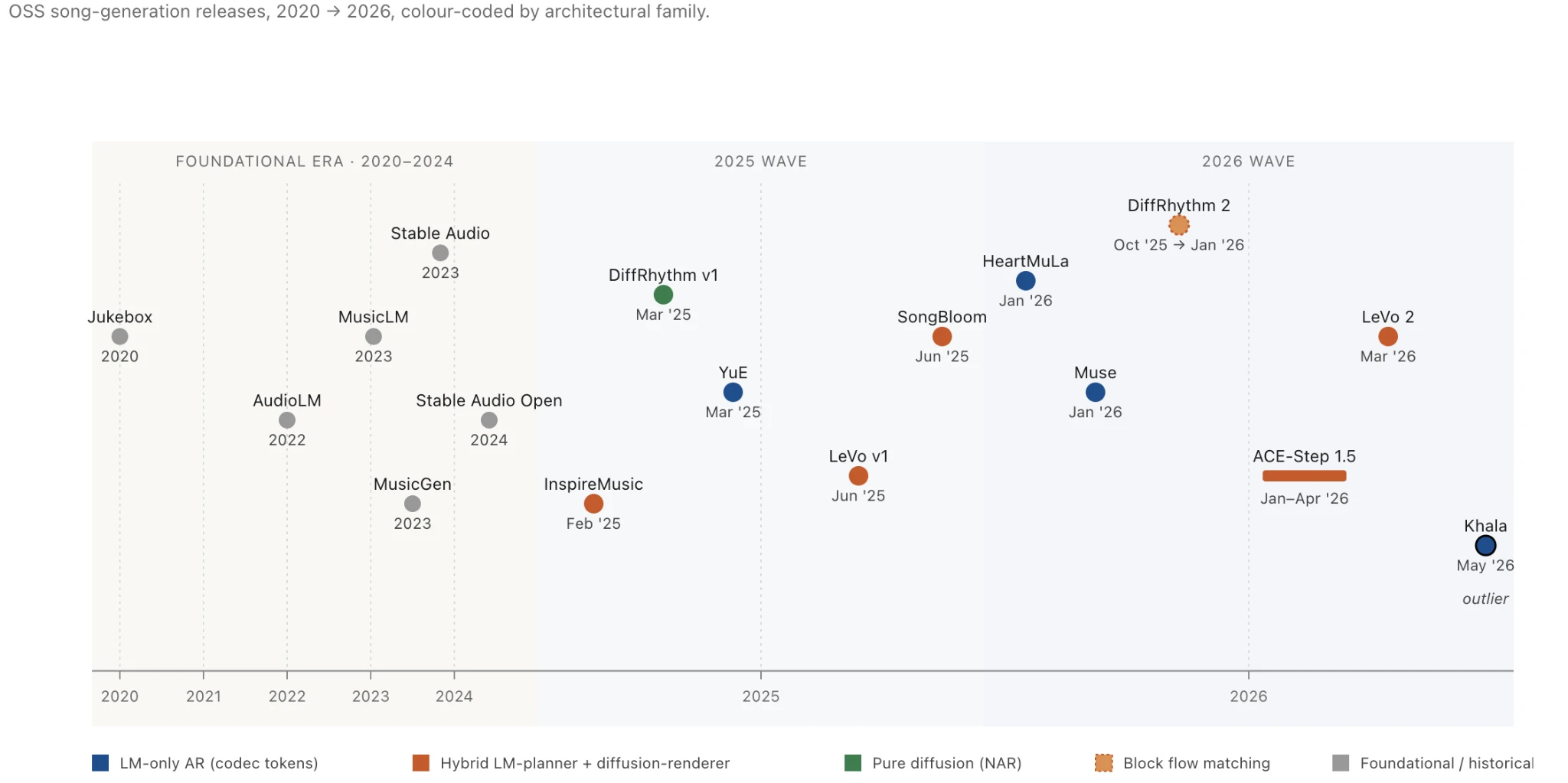
The timeline that produced the 2026 slate is short enough to walk in a single sitting, and walking it makes the rest of the post read more fluently. Figure 1 places every model on the same horizontal axis – and a handful of foundational works that came before them – colour-coded by architectural family. The two families that dominate the 2026 wave (LM-only autoregressive over codec tokens, and hybrid LM-planner plus diffusion-renderer) are visible as the two clusters at the right edge.
Things begin in 2020 with Jukebox (OpenAI), which set the basic recipe that subsequent open-weight music generation would either iterate on or deliberately depart from: hierarchical audio tokens, coarse-to-fine VQ-VAE, an autoregressive prior on top, lyrics conditioned through the AR backbone 🔗. Jukebox was big, slow, and impractical, but it established the engineering substrate the field has been polishing for six years.
AudioLM (Google, 2022) split the problem into semantic and acoustic tokens, treating music generation as a language-modelling problem over a learned audio vocabulary for the first time 🔗. MusicLM (Google, 2023) layered MuLan text-audio embeddings over that vocabulary and produced the first convincing text-to-music samples 🔗. MusicGen (Meta, 2023) compressed the recipe into a single-stage Transformer over EnCodec tokens, and shipped trained weights you could actually download and run 🔗. Stable Audio (Stability, 2023) and Stable Audio Open (2024) brought continuous-latent diffusion into the picture and contributed a music VAE that several 2026 open-weight models still use as their audio representation 🔗. The codec lineage that matters for what comes next runs EnCodec → DAC → MuCodec / X-Codec / Stable-Audio-VAE; the choice between them affects how a model sounds more than its parameter count does.
Meta was moving in a different direction at the same time: SAM Audio targets sound separation rather than generation, using much of the same diffusion substrate.
The 2025 wave is where the open community begins shipping models a practitioner can take seriously. DiffRhythm v1 (ASLP@NPU) made fast non-autoregressive diffusion practical for full-song generation, at RTF 0.034 on an RTX 4090 (around 28× realtime), with a phoneme-G2P lyric conditioning route that required sentence-start timestamps – one of the few details that still distinguishes the DiffRhythm line from the rest of the field, since almost everyone else moved to raw text 🔗. YuE (M-A-P) was the 7B LM-only system that quantified RoPE long-range decay and used that finding to justify segment-based conditioning, a pattern every subsequent full-song generator has since adopted 🔗. InspireMusic (Alibaba FunAudioLLM) brought a Qwen2.5 LM-planner over a flow-matching renderer into the open, though only its instrumental checkpoint shipped 🔗. LeVo v1 (Tencent SongGeneration v1) introduced the multi-stage DPO pipeline that LeVo 2 inherits and extends, with three separate offline DPO runs (lyric alignment, prompt consistency, musicality) merged by linear weight interpolation 🔗. SongBloom (Tencent and CUHK-Shenzhen) interleaved autoregressive planning with diffusion refinement and required a reference audio clip at inference, which is what puts it slightly outside the text-only comparison this post runs 🔗.
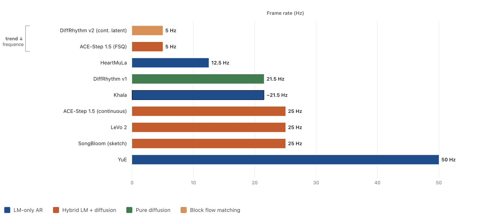
The 2026 wave, in roughly chronological order. HeartMuLa (institutional affiliation undisclosed in the paper) shipped early in the year with a multi-encoder codec (Whisper plus WavLM plus MuEncoder fused into a single 12.5 Hz quantizer, the lowest frame rate in the slate) over a hierarchical Llama-3.2-based LM with factorized DPO along the global/local seam 🔗. Muse (Fudan) followed with a deliberately vanilla 0.6B Qwen3 LM over MuCodec – no diffusion, no RL, no auxiliary losses; the contribution was not the architecture but the training corpus: 7,771 hours of fully synthetic Suno-V5 output, openly licensed, the only fully released training set in the slate 🔗. ACE-Step 1.5 (ACE Studio and StepFun) added an FSQ tokenizer to the v1 hybrid stack, shipped the most aggressive remix / edit / cover tooling in the field, and remains the only model whose alignment is fully intrinsic, with the DiT-side reward computed from its own attention geometry rather than a human-preference dataset 🔗. DiffRhythm 2 (Xiaomi Research and ASLP@NPU) introduced Block Flow Matching – non-autoregressive within blocks, autoregressive across them, KV-cached at the boundary – together with Cross-Pair Preference Optimization on 40,000 pairs in roughly 200 GPU-hours 🔗. LeVo 2 (Tencent SongGeneration v2) scaled LeVo v1 to about 4 B parameters and added a semi-online DPO stage with aesthetic scoring on top of the offline DPO base 🔗; the model arrived without a paper, and the technical report has been promised but not shipped. Khala (Central Conservatory of Music) is the year’s outlier, with a 64-layer-deep RVQ over pure acoustic tokens, no semantic stage, and a Task-0 hybrid-attention training trick standing in for the semantic conditioning every other model uses 🔗. The architecture revives Jukebox’s pure-acoustic-only thesis specifically – not the broader Jukebox influence on hierarchical audio tokens and the codec lineage, which is already visible everywhere above.
Two architectural families dominate that 2026 list, and the colour-coding in Figure 1 makes the split visible at a glance. The first is LM-only autoregressive over codec tokens, in which a transformer predicts the next audio token given lyrics and conditioning – YuE, HeartMuLa, Muse, and Khala live here. The second is hybrid LM-planner plus diffusion-renderer, in which an LM plans structure and a separate diffusion model renders frames – ACE-Step 1.5 and LeVo 2 live here. DiffRhythm 2’s Block Flow Matching belongs to neither cleanly; it is non-autoregressive within blocks and autoregressive across them, which makes it a hybrid by a different route. DiffRhythm v1 is the only remaining inhabitant of a third family that 2026 has otherwise left behind, pure non-autoregressive diffusion. The trade-offs each family makes – alignment cleanness, inference speed, audio fidelity, tooling reach – are what §3 walks through.
Which open-source model wins? A deep dive into each contender
We walk the slate in two passes. First, the three models that warrant a real deep-dive – the research substrate, the audio-quality winner, and the architectural outlier. Then six honorable mentions, each kept tight: enough to place the model and call out the one or two things that matter.
Is ACE-Step 1.5 the best open-source model for fine-tuning and remixing?
ACE-Step 1.5 is two things at once, and this section is going to walk both. It is the best target in the slate for fine-tuning, remixing, continuation, and any downstream work that benefits from a permissive license and rich tooling – by a margin large enough that there is no real second place. It is also the model whose audio carries the slate’s most distinctive artifact: a metallic shimmer we hear across the full runtime, on vocals and on instrumental sections alike. The architecture and the artifact share at least one suspect (the codec / tokenizer change between v1 and 1.5), which is why the model warrants a deep-dive rather than a one-line dismissal of either half.
Architecture. ACE-Step 1.5 is a hybrid LM-planner plus diffusion-renderer. A Qwen3-based LM sits upstream and produces a structured plan – BPM, key, duration, structure tags, lyric placement – and a DiT (around 2 B parameters in the standard variant, 4 B in 1.5 XL) renders audio frames given the plan 🔗. The audio representation pairs a custom 1-D VAE (Muon-trained) with an FSQ tokenizer operating at 5 Hz – among the lowest frame rates in the slate, in the same bracket as DiffRhythm 2 – and decodes to 48 kHz stereo. The MIT license covers both code and weights, and the HuggingFace model card carries a verbatim grant – “You can strictly use the generated music for commercial purposes” – that is unusually explicit for this field 🔗. We will return to the codec choice at the end of the section, because the tokenizer at 5 Hz is the load-bearing variable in our working hypothesis about the artifact.
The showpiece – intrinsic RL. This is where ACE-Step 1.5 does something nobody else in the 2026 slate does. Every other model that uses preference optimization (LeVo 2, HeartMuLa, DiffRhythm 2) needs preference data – pairs of (winner, loser) clips, labelled either by humans or by an external metric. ACE-Step 1.5 does not. Its reward signal comes from the model’s own internal state.
The intuition first, because the formal mechanism takes a paragraph to unpack. A DiT generating audio from lyrics learns a cross-attention map between the lyric tokens and the audio frames. If the model is doing its job, the map looks roughly like a diagonal stripe – lyric token n attends to audio frame m, with m increasing monotonically as n does. When the model goes wrong, the stripe goes wrong: it skips lyric tokens (gap), wanders backwards (singer goes out of order), or smears across many frames (alignment too fuzzy). ACE-Step’s training loop reads those properties off the attention map directly and turns them into a scalar reward.
The mechanism is called the Attention Alignment Score (AAS)🔗. It computes both directions of the attention map (lyric-to-audio and audio-to-lyric, so direction-consensus matters), then aggregates three sub-scores by Dynamic Time Warping: Coverage (did the singer sing every word?), Monotonicity (did the singer sing them in order?), and Path Confidence (how sharp is the alignment stripe?). The paper claims AAS correlates above 95% with human lyric-audio-sync judgements – a number we hold lightly because there is no before-and-after-RL PER ablation accompanying the claim, but the recipe is internally coherent. AAS feeds into a DiffusionNTF training loop, where DiffusionNTF is RL on diffusion via the forward noising process, which sidesteps the slow reverse-sampling-chain gradients that usually make RL on diffusion expensive 🔗. The LM side is GRPO with a Pointwise Mutual Information reward between generated captions and generated audio codes 🔗. Final LM reward weighting is 50% stylistic atmosphere, 30% lyric content, 20% metadata.
ACE-Step 1.5 is the only model in the slate whose alignment reward is defined by its own attention geometry. No human preference dataset, no external reward model, no third-party metric being optimized. RLHF without the H – reward from internal consistency, not from a downstream signal. The picture is unusual enough that, taken on its own, the paper would be a notable contribution to the alignment literature.
Omni-Task, because the foundation-model framing materializes here. The same DiT weights run six task modes via two knobs – what to condition on (Source Latent) and which output regions to overwrite (Mask) 🔗. The modes are text-to-music (synthesize from scratch), cover (re-synthesize timbre over an existing melodic skeleton), repainting (regenerate a time-window inside a track), track extraction (a generative stem separator), layering (add complementary instruments to an existing track), and completion (orchestrate a full arrangement from a single motif). No other 2026 model in the slate runs editing modes out of a single set of weights. The LM has four complementary modes – Planner (free text → structured YAML), Listener (audio → captions and lyrics, which is what makes the PMI reward possible), Co-Pilot (sparse query → full song structure), and Refiner (raw user input → canonical conditioning format) 🔗. Whether all four are exposed as user-facing endpoints or live inside the inference loop is not clear from the paper alone, but the framing is plain: ACE-Step 1.5 is positioned as a substrate, not a song-in-song-out service. That positioning is what makes it the research and fine-tune winner even though it is not the audio-quality winner.
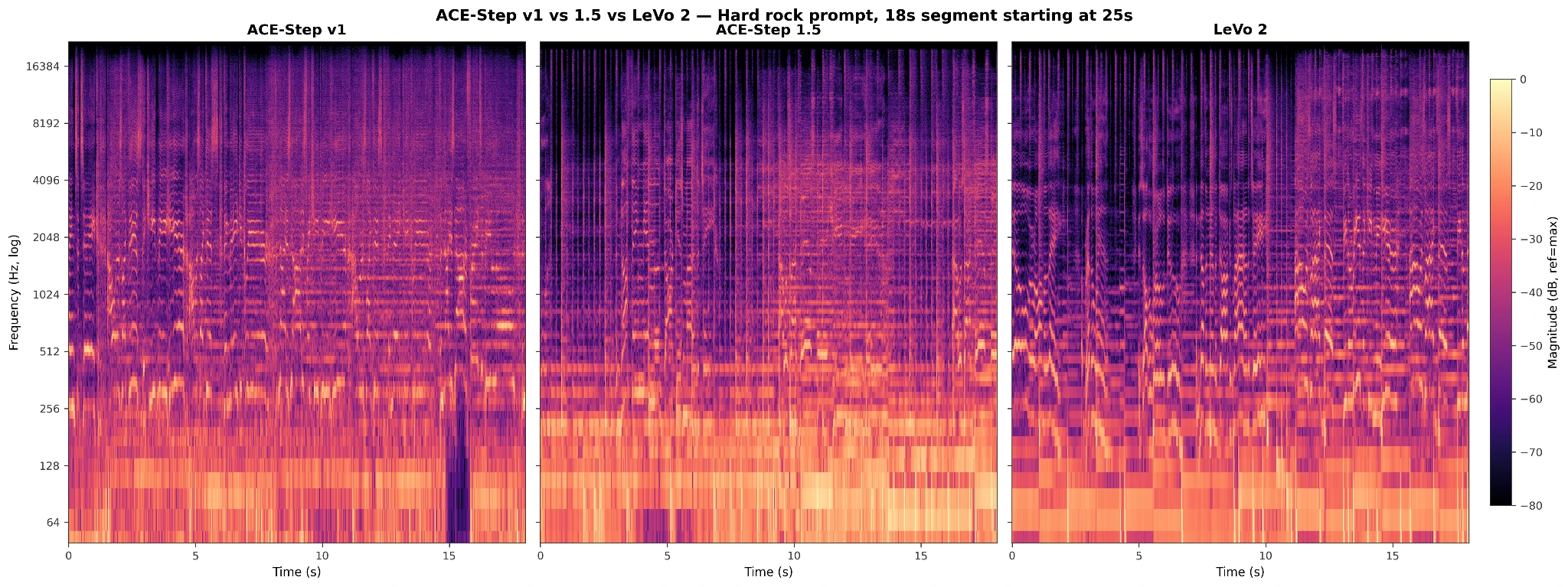
The audio verdict. ACE-Step 1.5 has a recurring metallic shimmer that we hear on sustained vowels and on cymbal-heavy instrumental passages alike. The cleanest place to hear it is the chorus of the Hard-rock sample around the second held “unknown” – the vowel tail goes glassy in a way nothing else in the slate does on the same prompt. Crucially, the artifact persists into the instrumental sections, which rules out the most obvious explanation (a vocal-codec-specific compression artifact). Our working hypothesis is that the artifact comes from either the DiT denoiser at low step counts or the FSQ tokenizer at 5 Hz – both are the components that changed between ACE-Step v1 and 1.5. We hold the hypothesis lightly: we have not done the obvious ablations (rerun the 1.5 weights with more diffusion steps, swap the FSQ stage), and we are working from listening, not from a controlled internal probe. What we do have is one piece of internal evidence pointing the same way: ACE-Step v1, which uses a different codec and tokenizer, does not have these artifacts. v1 trades that cleanness for weaker musicality. Figure 2 puts ACE-Step v1, ACE-Step 1.5, and LeVo 2 side by side on the same prompt; the spectrogram does not isolate the metallic character of 1.5 on its own, but the comparison to LeVo 2’s upper-band cleanness lines up with what the audio says.
If your work is fine-tuning, LoRA-training, downstream tooling, remixing existing tracks, or any pipeline that needs to extend the model rather than only call it, ACE-Step 1.5 is the right model in the slate. If you need pristine audio for end-user playback right now, the artifact will bother you, and the next deep-dive is the model you should keep reading for.
LeVo 2 review: does it produce the most natural-sounding AI music?
LeVo 2 is the quality winner of the slate, and the cost is the license. Across the three style-and-lyric combinations we tested, LeVo 2 produced the most organic and most natural-sounding clips of any model in the comparison; the verdict held on hard rock, on jazz, and on pop, and it is not the kind of verdict that depended on seed luck. The catch is that LeVo 2 ships under a Tencent custom license that forbids any commercial or production use, and that license arrives wrapped in some documentation noise we will untangle in a moment.
A note on documentation, because it shapes everything below. LeVo 2 is the only model in our slate without a standalone arXiv paper. The canonical documentation is the GitHub README, supplemented by the v1 paper for everything architectural that v2 inherits, plus a “technical report” that has been promised since 2026-03-01 and as of this writing has not shipped 🔗. Every load-bearing claim about LeVo 2 in this section carries the same caveat: vendor-self-reported, README-only, no third-party reproduction yet.
Architecture. LeVo 2 is a hybrid LM-planner plus diffusion-renderer, in the same family as ACE-Step 1.5 but from a different lineage. The LeLM transformer plans structure and lyric placement; a Music Codec DiT denoiser renders audio frames given the plan 🔗. v2 scales the LeLM to roughly 4 B parameters (from v1’s 2.136 B), though whether the 4 B refers to the LeLM alone or to LeLM plus the carried-over codec is not clarified in the README. Three inference VRAM tiers are documented for the first time in the LeVo line (10 / 22 / 28 GB), and maximum song length is 4 min 30 s.
License, verbatim – and the HuggingFace card is wrong. The Tencent custom license covers both v1 and v2 via a single LICENSE file on the main branch 🔗. The load-bearing clause: “You agree to use the SongGeneration only for academic, research and education purposes, and refrain from using it for any commercial or production purposes under any circumstances.” The grant explicitly excludes training data and “other AI components” from its scope, so reward models, annotation pipelines, and the aesthetic-scoring framework discussed below are not covered either. The HuggingFace model card for v2-large reads `— license: unknown —` because the weights are hosted on an individual account (`lglg666/SongGeneration-v2-large`) rather than under the Tencent organization 🔗. That is misleading at best; the actual license is the Tencent custom non-commercial described above, and anyone considering building on this model should read the LICENSE file, not the HF card.
The showpiece – the alignment pipeline. The reason LeVo 2 sounds the way it does is, almost certainly, the most aggressive preference-optimization pipeline of any model in the slate. LeVo v1 introduced multi-strategy offline DPO: three independent DPO runs along three preference axes (lyric alignment via ASR phoneme-error gap, prompt consistency via MuQ-MuLan similarity, musicality via a reward model trained on ~4,000 crowdsourced ranking seeds), and the three resulting fine-tunes were merged by linear weight interpolation🔗. The merge is the part worth noticing. Mixing the three preference datasets into one training run loses on most metrics – the gradient gets pulled in contradictory directions, because lyric alignment and musicality genuinely trade against each other. Training three separate models and combining them in weight space sidesteps that. The interpolation coefficient is exposed as a knob.
LeVo 2 keeps that base and adds a semi-online DPO stage with aesthetic scoring on top🔗. “Semi-online” is the new term and worth defining: standard DPO is offline – preference pairs are collected once and the policy never generates fresh candidates during training. Online DPO refreshes pairs every step, sampling fresh candidates from the current policy and scoring them on the fly (closer to PPO-style RLHF in cost). Semi-online sits between the two: the policy generates fresh candidates periodically, gets them scored, and refreshes the preference set, so the pairs reflect the current model’s distribution without paying for fully online sampling. The reward model used in this stage is not specified in the README; the most plausible candidate is the “Automated Music Aesthetic Evaluation Framework” that the same README lists as a TODO release, which would make the reward model a Tencent-team artifact, echoing the same-team-metric pattern v1 had with MuQ-MuLan.
The pipeline size moved with the strategy. v1 used roughly 60,000 preference pairs total across three axes; v2 reportedly uses about 200,000 pairs through the offline stage plus the periodic refresh in the semi-online stage. v2 reports PER 8.55% against Suno V5’s 12.4% on an undisclosed test set with an undisclosed ASR – a comparison we will not endorse without disclosure, but the broader point holds: LeVo 2 has had more, and more sophisticated, preference optimization applied to it than any other model we tested. That is plausibly why it sounds the way it does.
The audio verdict. LeVo 2’s clips sit in the mix the way recorded music does. The vocals avoid the metallic register that ACE-Step 1.5 falls into; the timbre work is plausible enough that on the jazz prompt it is not hard to forget for a few seconds that the take is synthetic; arrangements feel arranged, not interpolated. We do not have an ablation that isolates which part of the alignment pipeline did which work, but the pattern is consistent enough that we will say it plainly: among the eight models in our experiments, LeVo 2 is the one whose output we would most confidently call music rather than a generated audio file. The price of that verdict is the license. If you can live inside academic, research, or education use, LeVo 2 is the model to use. If you cannot, the verdict still stands, but the model that wins on quality is not the model you can ship.
What makes Khala the most architecturally unusual model in the 2026 slate?
Disclaimer the authors pinned to the repository as of May 2026: We have identified a potential issue that may significantly affect inference quality. The problem is currently under investigation and may be related to numerical precision. Until this notice is removed, please treat current generation quality as unstable.
Khala is the most architecturally distinctive thing the 2026 wave produced, and the audio – even under the disclaimer – is doing something none of the other models do. In some cells, the model produces melodies and vocal motifs that nothing else in our slate produces; in others, the audio comes out structurally simple in a way that pulls the listening verdict back toward the disclaimer. The architecture is interesting enough that the deep-dive is worth writing under provisional listening, and we will revisit the verdict if the fixed release changes the picture.
Khala is the only 2026 model that revives Jukebox’s pure-acoustic, no-semantic-stage thesis 🔗. The precision matters because Jukebox’s broader influence – hierarchical audio tokens, coarse-to-fine RVQ-style coding, the whole EnCodec → DAC → MuCodec lineage that runs through the field – is felt across every model in the slate, including the ones that are otherwise nothing like Jukebox. What Khala specifically revives is the part that consensus walked away from: doing music generation in acoustic-token space only, with no semantic-token stage between the lyrics and the audio frames. Every other model we tested (YuE, HeartMuLa, Muse, ACE-Step 1.5, LeVo 2, DiffRhythm 2) uses semantic tokens, a diffusion-based renderer, or both, on the assumption that pure acoustic-token autoregression hit a ceiling at the Jukebox scale for reasons that should not be re-litigated. Khala bets those reasons were wrong, or at least worth retesting now that codecs and compute have moved on by six years.
Architecture. Three networks in series, with a total parameter budget that lands mid-pack for the slate. A 1.6 B-parameter backbone autoregresses over the coarsest RVQ layer – the layer carrying most of the structural information. A 1.8 B-parameter super-resolution stage fills in the finer RVQ layers above the coarse one. A 0.27 B-parameter codec handles the encode-and-decode round-trip 🔗. Total: roughly 3.7 B parameters across the three. The interesting number is the codec depth – Khala runs a 64-layer-deep RVQ, which is the deepest in our slate by a substantial margin. Deep RVQ buys reconstruction fidelity at the cost of longer token sequences to predict, and the bet behind 64 layers is that the depth lets the autoregressive backbone work in pure acoustic space without needing a separate semantic abstraction to hold the structure together.
The mechanism standing in for the semantic stage everyone else uses is Task-0 hybrid attention🔗. During training, the model runs two attention modes side by side: causal attention for a Task-0 lyric-alignment objective (the model has to predict lyric tokens in time-aligned position alongside audio tokens), and full attention for layer-wise audio refinement. At inference, Task-0 is not used; it is a training-time architectural induction, not a separate forward pass. The framing in the paper is that this lets text-and-vocal alignment emerge without an explicit semantic bridge, the way that bridge would exist in a model running a HuBERT or W2V-BERT semantic stage between lyrics and audio. Whether the trick actually compensates for the missing semantic stage is the empirical question Khala exists to answer.
The training corpus is the second distinctive piece, and worth a paragraph on its own. Khala was trained on roughly 18 million tracks comprising 1.2 million hours of audio, drawn from the Central Conservatory of Music’s internal music dataset 🔗. The hours number is the largest in our slate. The more interesting fact is that this is a different species of training data from everything else in the field – an institutional music-conservatory archive rather than scraped Internet audio. Provenance is documented at the institutional level (conservatory dataset, internal use) but not per-track; better than the “we say nothing” pattern most papers fall into, not as transparent as Muse’s fully published synthetic corpus. The contribution worth flagging on its own terms: conservatory archives are a different bucket of training data, with a different stylistic distribution, a different acoustic provenance, and a different legal posture from the audio scrapes everyone else trains on. Seeing a 1.2 M-hour model trained from one is unusual, and we are interested in what training on archive-grade audio specifically buys.
License. Khala ships under CC BY-NC 4.0 – non-commercial like LeVo 2, but for different reasons (conservatory data provenance and institutional norms rather than corporate IP).
The audio verdict, under the disclaimer. Khala has a noticeable AI character that we hear in the arrangements first. Many of the generations come out structurally simple, light on harmonic motion, light on the rhythmic risk-taking that gives generated music a sense of personality. The model is also genuinely unstable run to run, and the intros are often messy in a way none of the other models in the slate are – the first few bars take time to find their footing, which is consistent with the failure mode the authors are warning about. Vocals are not consistently expressive across cells; some are flat in a way that reads as obvious model-output. A few generations also have natural-sounding voices that compare favourably to the deep-dive winners. LeVo 2 still wins aggregate audio quality across the cells we have, but Khala is not a model to dismiss: the bet on deep-RVQ pure-acoustic autoregression is producing genuinely different output on some prompts, and the disclaimer suggests the current state of the model is not its ceiling. The messy intros and run-to-run instability read as likely to improve with future code updates, which is also what the disclaimer is pointing at.
To close, Khala is the architectural outlier of the 2026 slate: a different bet from everyone else, with audio that supports the case on some cells and undermines it on others, and with the disclaimer still attached. The license keeps it out of commercial product work alongside LeVo 2. For research, for understanding where the field could still go, and for anyone interested in routes through music generation that the consensus has closed prematurely, Khala is the model to pay attention to over the next six months.
How do YuE, HeartMuLa, Muse, and DiffRhythm 2 compare?
YuE (M-A-P, Apache 2.0) is the 2025 lineage anchor of the 2026 wave and the place to start a careful honorable-mentions read 🔗. Its paper did something rare in this field – it quantified the failure mode it was solving. The claim that “degradation begins around 3K tokens, complete failure beyond 6K tokens” without chain-of-thought conditioning is what justifies the segment-based conditioning recipe (~14 sections per song, ~30 s each, with text plus lyrics plus audio interleaved per section) that every post-YuE full-song generator has since adopted. The paper also includes a Limitations section that names its own failure modes, which is the kind of behaviour we would like to see more of in the field. The license is Apache 2.0 with an explicit commercial-use grant.
The listening verdict is less generous than the lineage credit. YuE’s audio did not stand out on quality or musicality across the three styles we ran; the more practical drawback is inference speed. On an RTX 4090, YuE runs at roughly 12× slower than realtime, which makes running a small experimental sweep a noticeable time cost – and over a long enough horizon, time cost is itself a quality cost, because it bounds how much prompt iteration you can afford. Community forks (YuEGP, YuE-exllamav2) exist precisely because of this.
HeartMuLa
HeartMuLa (Apache 2.0 code) is the slate’s interesting-codec model with a less-interesting audio verdict 🔗. The novel contribution is the codec design: HeartCodec runs at 12.5 Hz – the lowest frame rate in the slate – and fuses three encoders (Whisper plus WavLM plus MuEncoder) into a single quantizer. Most music codecs use one encoder; HeartCodec’s bet is that mixing semantic-leaning encoders with an acoustic one yields a richer token distribution. The LM on top is Llama-3.2 in a hierarchical Global plus Local configuration, with DPO factorized along the global / local seam – clever paper-craft, empirical lift over a monolithic DPO baseline left unmeasured.
Our listening verdict: HeartMuLa sounds the same across styles. We tried hard rock, jazz, and pop, and what came back was generic pop in every case – averaged, smoothed, AI-blurry. We frame this carefully, because it could be a weights or inference quirk on our end, but the consistency across all three prompts pushes the explanation toward something structural in the released checkpoint. One small note for the careful reader: HeartMuLa’s abstract claims significant gains at 7 B parameters, but only 3 B SKUs ship.
Muse
Muse (Fudan, MIT code, Apache-2.0 weights, MIT data) is in the slate for one reason that has nothing to do with its architecture and everything to do with its training data 🔗. The model itself is deliberately vanilla – a 0.6 B-parameter Qwen3 over MuCodec, single-stage SFT, no diffusion, no RL, no auxiliary losses. The paper says this in so many words: “without task-specific losses, auxiliary objectives, or additional architectural components.” The bet is not on the model; the bet is on the corpus: 7,771 hours of fully synthetic Suno-V5 output, generated by Suno V5 plus GPT-5-mini plus Qwen3-Omni-30B, released MIT, the only fully released training corpus in the slate. If you want to train a competitor on the same data, you can. That is the contribution.
The headline claim – that 0.6 B Muse beats 8 B YuE on every column of a SongEval benchmark – does not survive a careful reading: the test set is 100 songs, there are no confidence intervals, and SongEval is published by a different team that is itself a competitor (DiffRhythm). We will not endorse the “beats YuE” framing. What our own listening said is more modest: Muse’s general audio quality is better than ACE-Step 1.5 in the cells we ran, and the model produces audio with a distinct Chinese-leaning “accent” on English-prompt vocals – most plausibly because the synthetic corpus was Chinese-curated even though Suno V5 was the synthesis engine. The legal hinge worth flagging: Muse’s openness rests on Suno’s terms of service permitting this kind of derivative use, and the paper does not engage that question.
DiffRhythm 2
DiffRhythm 2 (Xiaomi Research and ASLP@NPU, Apache 2.0) is the architecturally most novel thing in the 2026 slate, and also the slate’s most paper-honest model 🔗. The architecture is Block Flow Matching: split the latent into blocks of about two seconds, denoise within each block in parallel (the non-autoregressive part), and condition each block on all previous clean blocks via KV-cached attention (the autoregressive part). The result is semi-autoregressive – fast within a block, structured across blocks, with KV caching at the block boundary keeping inference cheap. The alignment recipe is Cross-Pair Preference Optimization on 40,000 pairs in roughly 200 GPU-hours total, which is strikingly small for an open-source state-of-the-art claim (the GPU type is not named).
The audio verdict has two halves. On the positive side, DiffRhythm 2 has the lightest style-impact across genres of anything in our slate – different style prompts genuinely produced perceptibly different-feeling generations, which is harder than it sounds and several models in this list fail at. On the negative side, the audio is more artificial than the deep-dive winners, the rhythm is genuinely unstable (which is a quietly funny finding given the model is named DiffRhythm), and the paper itself flags vocal quality as behind ACE-Step and LeVo in §5.2. One possible cause of the rhythm instability that we offer as a hypothesis rather than a finding: DiffRhythm 2 is among the few models still using phoneme-based lyric conditioning, and phonemes strip prosodic and timing cues that raw-text models retain. The most useful thing we can say about DiffRhythm 2 is that its paper says what is wrong with it without our needing to ask: §6 contains the “Open-source still falls short of commercial systems overall” line that the rest of our post borrows as a thesis quote, and §5.2 admits the vocal-quality gap to ACE-Step and LeVo directly. Vendor-side honesty of this kind is rare, and it earns the model the credit we are giving it here.
Frames per second of the audio representation each model’s LM (or diffusion) operates on. Some are discrete codec tokens; others are continuous VAE latents — the relevant axis is the same.
How do you evaluate AI-generated music quality?
Song generation is harder to evaluate than text-to-speech, and nobody has settled on what good evaluation looks like yet. Our own pass is small: three style-and-lyric prompts at one seed per model, what a practitioner with a cheap GPU and a week to listen would actually manage. Not a benchmark. A practitioner’s pass.
A text-to-speech system can be scored by intelligibility, which is roughly a scalar: did the listener understand the words? A song-generation system has to be scored on intelligibility and on musicality, mix balance, emotional fit, style adherence, structural coherence, vocals creativity, and how the vocals sit against the instrumental. Most of these resist single-scalar measurement, and many of them interact – a vocal that is more intelligible may be less expressive, a mix that is cleaner may be flatter, an arrangement that adheres more tightly to the prompt may be more boring. There is no current benchmark that captures the whole picture cleanly, and the ones that try are doing real work by trying.
The WER caveat that almost every paper buries. Almost every paper in this space reports a Word Error Rate or a Phoneme Error Rate as a load-bearing intelligibility metric. WER and PER are computed by running an ASR over the model’s outputs and comparing the transcript to the lyric input. The catch – and the reason careful readers should treat WER as a soft signal – is that the ASR is itself a model with its own failure patterns. A model that produces audio the ASR happens to like will get a better WER than a model that produces audio the ASR happens to find unfamiliar, regardless of how intelligible the audio is to humans. We have heard cases where a model with a better-reported WER is subjectively less intelligible to a human listener than a model with worse-reported WER. The right reader habit is to ask which ASR was used and how it was chosen.
Subjective surveys are still the best signal, and consistently underpowered. The single most useful thing a paper can do is run a properly powered subjective evaluation: enough raters, blind to model identity, with explicit rating dimensions, scored across enough samples that fatigue does not dominate the result. Most papers in this space ship subjective evals with 9 to 40 raters per metric, which is enough to spot a large effect and not enough to distinguish close calls. LeVo v1 used 10 paid professionals across 20 lyrics × 3 modes. HeartMuLa used 9 raters across 20 samples. YuE used about 40 evaluators with an unexplained split. DiffRhythm v1 used 30 listeners. DiffRhythm 2 used 10 pro listeners. Muse used zero humans – all of its headline metrics are automatic. These are not bad numbers for the constraints, but anyone reading the resulting tables should know what those constraints are.
SongEval, SongBench. Two benchmark efforts in this space deserve real credit. SongEval (published by the DiffRhythm team at ASLP@NPU) is the closest thing the field has to a shared subjective-evaluation framework, and several 2026 papers report numbers on it as a load-bearing metric: ACE-Step §5.1, DiffRhythm 2 §5.1, HeartMuLa Tables 7–11, Muse §5.3. SongBench plays a similar role for parts of the slate. Building benchmarks is mostly thankless work; the only reason the model teams are also the benchmark teams is that nobody else is doing it.
Four of the eleven Tier-A 2026 models report SongEval numbers, and SongEval comes from one of those eleven teams. MuQ-MuLan, which LeVo uses as a headline text-audio similarity metric, is a Tencent same-lab artifact. HeartMuLa’s PER pipeline uses HeartTranscriptor, which is HeartMuLa’s own ASR – the same ASR is used to compute (a) HeartCodec’s WER table, (b) HeartMuLa’s PER table against competitors, and (c) the reward signal for one of three of its DPO sets. None of these patterns mean the numbers are wrong. They mean that reading those numbers should include the question of who built the metric, alongside the question of what it measures.
Benchmark tables are one half of the evaluation problem. The other half is knowing what those benchmarks are measuring on, and that question hits a wall almost immediately.
Of the eight models in our slate, exactly one (Muse) releases its training corpus.
Every other paper either omits training data entirely, names it only at an institutional level (Khala’s “internal music dataset”), or acknowledges internet-sourced material whose provenance no one can audit.
The field’s training-data opacity is its most structural problem, and no single model team can fix it. No one is obliged to. But anyone running a comparison is implicitly trusting eight different opaque pipelines, and that trust has no verifiable floor.
One clean direction toward solving this is licensed synthetic data: training corpora generated by other models whose outputs the trainer has clear legal rights to use, with documented generation pipelines and released datasets. Muse demonstrates the basic shape – generate audio with Suno V5, lyrics and prompts with GPT-5-mini, refinement with Qwen3-Omni-30B, release everything MIT.
Open-source music generation models compared: full listening results
Prompts
Hard rock
Jazz
Pop
Hard rock anthem. Male lead vocal with grit and edge — rough but melodic, not screamed. Distorted electric guitars: palm-muted single-note riffing in verses, full power chords in choruses. Driving bass, energetic 4/4 drums around 140 BPM, cymbal crashes on chorus downbeats. Anthemic shout-along chorus. Brief guitar lead between sections.
Show lyrics
[Verse 1]
The streetlights bow their heads to let me through
The sky has spilled its silver on the lake
A breath of wind is all the world will do
And nothing in the dark is mine to take

[Pre-Chorus]
Hours like this, they keep me here
Hours like this, they make it clear

[Chorus]
The night is not afraid to be alone
The night is not afraid to be unknown
And every quiet thing I cannot say
Is somewhere in the way the stars are sown

[Verse 2]
A window glows above an empty street
A radio is humming through the wall
The world has slowed enough that I can meet
The smaller part of me beneath it all

[Pre-Chorus]
Hours like this, they keep me here
Hours like this, they make it clear

[Chorus]
The night is not afraid to be alone
The night is not afraid to be unknown
And every quiet thing I cannot say
Is somewhere in the way the stars are sown

[Bridge]
And nothing has to happen for it to be enough
Nothing has to ask, nothing has to hush
Just the slow way midnight breathes in time
With a soft and sleeping town

[Chorus]
The night is not afraid to be alone
The night is not afraid to be unknown
Smooth jazz quartet. Intimate male crooner vocal — warm, conversational, slightly behind the beat. Walking upright bass, brushed drum kit, warm Rhodes electric piano comping, muted trumpet fills between vocal phrases. Moderate swing, around 95 BPM. Late-night club atmosphere. Tasteful reverb, no compression sheen.
Show lyrics
[Verse 1]
Don't search the lines for any hidden truth
These words were written purely as a test
No subtle code, no clever reverse-proof
Just syllables to hear if it sings best

[Pre-Chorus]
So close your notebook, set the verdict aside
Just listen, listen, listen for the ride

[Chorus]
There is no message, just a melody
Don't read between the lines you hear
The soul of song is sound, you must agree
Let go the meaning, let the music make it clear

[Verse 2]
A poet would be jealous, I'm aware
But poetry is not what we are after
We're checking if the model holds the air
And if the chorus gives a little laughter

[Pre-Chorus]
So close your notebook, set the verdict aside
Just listen, listen, listen for the ride

[Chorus]
There is no message, just a melody
Don't read between the lines you hear
The soul of song is sound, you must agree
Let go the meaning, let the music make it clear

[Bridge]
The lyrics here are scaffolding
For voices we are testing in the dark
Don't take them home, don't take them anything
Just check the pitch, the timbre, and the spark

[Chorus]
There is no message, just a melody
Don't read between the lines you hear
The soul of song is sound, you must agree
Let go the meaning, let the music make it clear
Modern pop ballad. Female lead vocal — breathy delivery in verses, controlled belt in the chorus. Mid-tempo, around 100 BPM, 4/4 time. Layered synth pads, crisp 808 kick with finger-snap percussion, clean electric guitar arpeggios, airy reverb tail, polished radio-ready mix. Melancholic verses lifting into uplifting chorus. Subtle vocal harmonies in the chorus.
Show lyrics
[Verse 1]
We taught the silence how to sing
Fed it words and watched them turn to light
Every echo learns a different thing
Stories that the wires hold tight

[Pre-Chorus]
Now the static finds a melody
Now the data finds a rhyme

[Chorus]
Hear the future humming low
Through the wires, soft and slow
Voices we did not compose
Sing us back to who we know

[Verse 2]
A thousand models reaching for a tune
Some get lost and some come dancing through
Half a moonbeam, half a chip-design
Half the heart is yours, the rest is mine

[Pre-Chorus]
Now the static finds a melody
Now the data finds a rhyme

[Chorus]
Hear the future humming low
Through the wires, soft and slow
Voices we did not compose
Sing us back to who we know

[Bridge]
Maybe music never needed hands
Maybe it was waiting in the strands
Patient as a dream
Patient as a flame

[Chorus]
Hear the future humming low
Through the wires, soft and slow
Voices we did not compose
Sing us back to who we know
The listening table
Model
Hard rock
Jazz
Pop
License
LeVo 2
Tencent (non-commercial)
ACE-Step 1.5
MIT
ACE-Step v1
Apache 2.0
Khala
CC BY-NC 4.0
DiffRhythm 2
Apache 2.0
Muse
MIT code / Apache 2.0 weights / MIT data
HeartMuLa
Apache 2.0
YuE
Apache 2.0
Which model should you use? The verdict
LeVo 2 wins on audio quality.
The verdict held across all three style-and-lyric combinations: hard rock, jazz, pop. The clips are the most natural-sounding clips of any model in our slate, by a margin that does not require a careful listening pass to detect. The cost is the Tencent custom non-commercial license, which forbids any commercial or production use. If you can live inside academic, research, or education use, LeVo 2 is the model you should use; if you cannot, the verdict still stands but the model you use is going to be a compromise.
ACE-Step 1.5 wins on research, fine-tuning, and downstream tooling.
The MIT license on code and weights, the Omni-Task editing modes, the documented architecture, and the maturing community ecosystem make it the substrate of choice for anyone building beyond a single model call. The cost is the metallic shimmer artifact we discussed in the deep-dive – audible on vocals, audible on instrumental, persistent enough across runs that it is structural rather than accidental.
Khala is the architectural outlier worth listening to.
A different bet from everyone else in the slate (pure-acoustic, no semantic stage, 64-layer-deep RVQ) producing audio that is sometimes genuinely interesting and sometimes structurally simple, all under an active stability disclaimer. The cost is two-part: the disclaimer says the current state is unstable, and the CC BY-NC 4.0 license keeps the model out of commercial work alongside LeVo 2.
Any verdict in this section will age. Some of these models are improving in real time – Khala in particular is mid-stabilization as we write, and a fixed release could reshuffle parts of the table – and the headline next-release cycle will not slow down.
Will open-source models ever close the gap to Suno?
Between 2024 and 2026, the open community built something that did not exist before: a set of models where a careful listener can occasionally mistake the output for a real recording. That happened faster than most of the field expected. The gap to Suno has not closed.
Two things keep it open, and neither is close to resolved. Training data is the harder one: the volume of music that carries a license permitting neural-network training is small, and that is not changing at any speed. The research community knows this and is working in the direction it can: leaner architectures, tighter pipelines, more from smaller corpora. Compute is real too; training any of these models from scratch sits at a cost that limits who can do it. Both constraints point the same direction: clean corpora used well, not large ones used opaquely.
We do not expect open weights to close the Suno gap cleanly. What we expect is steady architectural improvement. The shift that matters more long-term is open architectures that teams can train on data they actually own, not open weights trained on data no one else can audit or replicate. That is a different kind of open, and probably the more useful one.
IT-JIM builds music and audio AI for products: pipelines, fine-tuned models, plugin integrations. Song generation is useful well beyond end-to-end generation; it is also the foundation for editing tools and creative interfaces that no vendor API will expose. If you are deciding whether one of these models belongs in something you are building, and the evaluation in this post is not deep enough for that decision, that is the kind of work we do.
Today, there is almost no digital field where 3D assets haven’t found their place: CGI, games, VR/AR, physics simulations, fashion design, marketplace product renders – you name it. Over the past decades, this spread into everyday life and transformed the 3D modeler role from a programmer in an engineering lab to an artist using specialized software.
With the controversial, yet revolutionary AI advancements in generating text, images, video, and music, it seems only natural that 3D generation should be product-ready out of the box, requiring at most a thin wrapper over an API call. But, here’s the twist: that is simply not the case.
So, how big is the gap between expectations and reality in AI-based 3D asset generation exactly, and is there a way to breach it right now?
Expectation
Real Inference
What Makes a 3D Asset Usable? Geometry, Materials, and Metadata
Let’s start from afar. The concept of 3D assets didn’t spring from computer science alone. The first mentions in a modern context date back to the Bézier curves that French automotive engineers came up with in the 1960s, followed by… Okay, stop. Maybe this is too far away from what we need.
What we really need is to understand how to represent the spatial position of an object, as well as its relevant properties, conveniently. Akin to 2D image raster and vector formats, there are two approaches for storing spatial information.
Meshes are the 3D equivalent of the raster format. We describe objects with determined blocks, but instead of a pixel, the minimal building block here is a polygon in a 3D coordinate system, usually a triangle, though sometimes a 4-corner shape (quad) is more convenient. A single point of a mesh is called a vertex, a connection between two vertices is an edge, and a group of connections that form a closed polygon is a face. Simple enough. Meshes are used when artistic control, organic shapes, or real-time performance is required. Few of the typical formats for them are OBJ, STL, and FBX.
On the other hand, analogous to vector 2D images, we have CAD-like formats. These use precise, parametric, mathematical definitions (NURBS), which are the evolution of the Bézier curves we mentioned earlier. Use CAD when dimensions and manufacturing precision matter (STEP, IGES, SolidWorks). Native CAD generation and AI mesh-to-CAD converters aren’t even close to production-ready yet, so we’ll leave them off the table for now.
We covered geometry, but it’s merely the skeleton; to become a functional 3D Asset, it must be fleshed out with properties. Visual realism standard is Physically Based Rendering (PBR), which defines metalness and roughness of the material, not just color, while interactivity demands physical data like collision bounds and rigging. Without this metadata, a generated model is just a static mathematical shell, not a usable item for a game engine.
This “packaging” step is the true bottleneck. While AI can easily hallucinate an acceptable raw shape, it struggles to organize it into complex production formats (like FBX or USD) that bundle geometry, materials, and hierarchy together. The gap between “Expectation” and “Reality” lies here: users want a plug-and-play asset, but AI currently delivers only the raw, unpolished geometry.
CAD
Mesh
How AI 3D Generation Works: From a Photo to a Mesh
A “3D generation model” is rarely a single model; it is usually a complex AI system comprising several specialized networks and pre/post-processing scripts disguised under a shared name. It takes a simple input (like a text prompt or an image) and attempts to return usable geometry and textures. To understand what is actually going on under the hood, we have to look at shape and appearance separately, as they are traditionally treated as sequential tasks. We’ll look at this from the “How it started vs. How it’s going” angle.
Brief historical overview
Initially, acquiring 3D shapes was a pure engineering challenge. Techniques like Structure from Motion (SfM) and Multi-View Stereo (MVS) relied on handcrafted feature detectors (like SIFT, Lowe 2004) to mathematically triangulate points from hundreds of high-overlap images.
The Deep Learning Era shifted this approach. 3D-GANs (Wu et al., 2016) attempted to map 2D images directly to 3D voxel grids, but they hit a “cubic memory wall”: doubling the resolution increased memory usage by eight times. A workaround occurred along with Neural Radiance Fields (NeRF) in 2020: by focusing on novel view synthesis, the network learns to “picture” the object from any direction rather than storing its physical volume. With these generated views, it boils down to classic reconstruction tools mentioned earlier to create a mesh, removing the need for the network to handle complex 3D geometry directly. Our separate NeRF in 2023: Theory and Practice guide covers the full training and rendering workflow in NeRFStudio, including the limitations that pushed the field toward generative methods.
All these experiments across a couple of decades laid the groundwork, but practical 3D generation required a fundamental shift in approach. The generative branch began sprouting with DreamFusion (Poole et al., 2022). It introduced Score Distillation Sampling (SDS), allowing 2D diffusion models (like Stable Diffusion) to “judge” and optimize a 3D shape until it looked correct from every angle. This was “dreaming” 3D from 2D priors and was painfully slow, but it was the final missing piece that allowed for revolutionary progress.
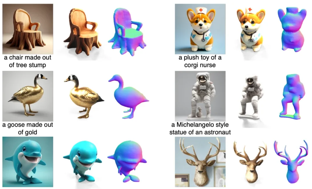
So, by 2022, the paradigm itself has changed. 3D generation was no longer the deterministic triangulation problem of the SfM era, which demanded lots of multi-view data. Instead, the neural networks were taught some degree of 3D space awareness, even if via indirect means. With these semantic priors, as little as a single image can be turned into a mesh. Unfortunately, the quality of those generations was far from being useful.
Unsettling DreamFusion generations
Path to The Modern Generation
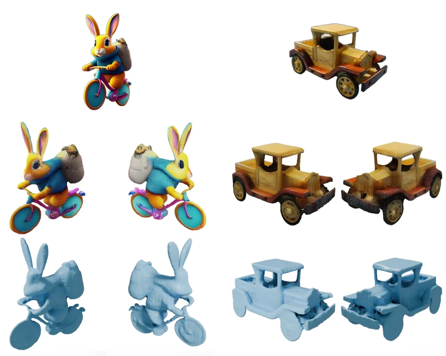
With all priors set up, a major practical shift followed in 2023 with the rise of multi-view diffusion. As the 2D generation already showed great results, researchers tried “forcing” those models to understand 3D. Zero-1-to-3pioneered this by fine-tuning Stable Diffusion on camera angles and 3D data, while One-2-3-45++ later fleshed out the concept into a complete 3D mesh generation pipeline.
One-2-3-45++ generations
Building on this in late 2023, the LRM architecture pioneered a family of Large Reconstruction Models, enabling near-instant, feed-forward generation. In this workflow, a 2D diffusion model first generates 4-6 consistent views from a single image, which LRM “stitches” into a Triplane-NeRF in about five seconds. The mesh still needs to be extracted via an algorithm like Marching Cubes, but the overall speed-up was impressive. While models like InstantMesh (2024), TripoSR (2024), and Hunyuan3D v1.0 (2024) refined this process, they couldn’t overcome the inherent flaws of Triplanes. Because Triplanes rely on 2D axis-aligned projections, they struggle with complex “concave” geometry or occlusions. Furthermore, if the initial views lack perfect pixel-alignment, the 3D output collapses into a blurry mess. Finally, Triplanes suffer from quadratic memory scaling: the same problem as earlier approaches faced with a 3D voxel grid, but less severe. All these capped the level of detail these models can achieve and their further development.
InstantMesh generations
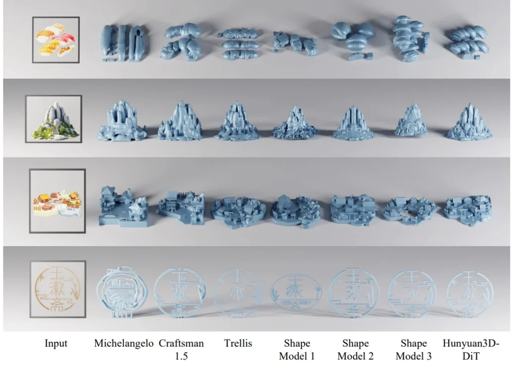
This path of trial and error leads to the current state-of-the-art: the Native 3D Era (Late 2024-Present). These models generate assets directly in high-dimensional latent space, skipping the “stitching” phase and the “memory wall” entirely, much like how modern 2D models create images. Two families currently lead the field. The TRELLIS Family prioritizes topological flexibility; its latest version utilizes compact structured latents (SLAT) to encode geometry and PBR materials into a sparse grid. By being “field-free” (moving away from Signed Distance Fields (SDFs), which earlier models in this class used), it can represent complex, non-manifold geometry like open clothing or thin leaves with ease. Meanwhile, the Hunyuan3D Family focuses on massive scale and precision. Hunyuan3D v3.0 leverages a 10-billion-parameter (vs nearly 4 in the latest Trellis) Diffusion Transformer (DiT) to treat 3D generation like a language problem, using a hierarchical “sculpting” approach. It generates a global coarse shape first and progressively refines it to ultra-high resolutions, effectively eliminating the surface noise and artifacts that plagued earlier generations.
Hunyuan3D v2.0 shapes comparison with analogs
Texture & Material Generation
Once the shape is solidified, it needs to be colored. Historically, this meant projecting 2D images onto a mesh (Texture Mapping). Early models like TRELLIS 1 and Hunyuan 2.0 treated this as a separate, decoupled task, which often resulted in a “plastic” look and noticeable texture drift. Modern versions have shifted toward Native PBR Generation, predicting Albedo, Metalness, and Roughness simultaneously by analyzing both the input image and local geometric details like curvature or sharpness.
TRELLIS 2 utilizes Structured Latents to predict material parameters for specific 3D points directly. By generating material tokens that are perfectly aligned with geometry tokens within the same grid, the materials are “baked in.” This provides superior localization, preventing “bleeding” between different surfaces (think about keeping a gemstone’s high-gloss shine strictly separate from a matte metal ring).
Hunyuan 2.1/3.0 uses a Sequence-based Latent instead of a fixed grid, so they came up with Mesh-Conditioned Multi-View Diffusion. It essentially “paints” the asset by observing the geometry from multiple angles. To solve the localization problem, it injects 3D coordinates into the 2D process using Normal Maps, CCM, and 3D-Aware RoPE. This ensures the model recognizes a single 3D point across different views. They also keep color and material data in parallel branches that stay synchronized through shared attention.
Hunyuan3D vs TRELLIS: Comparing the SOTA AI 3D Generation Models
A model’s true value often depends on its adaptability. While proprietary systems often work well out of the box, you have no means to customize them for niche requirements. Having identified the SOTA comes down to two leading “Native 3D” families, the next question is accessibility. How open are these systems? TRELLIS is completely open-source. Both training and inference code are available, making it very developer-friendly. On the contrary, Hunyuan3D v3.0 is currently closed and available only via API. Its predecessor, v2.1, has released weights and code, but the training script requires significant tweaking to work reliably (or at least work at all), so we can consider it an “open-weights” model at best.
Input image
Generated 3D still
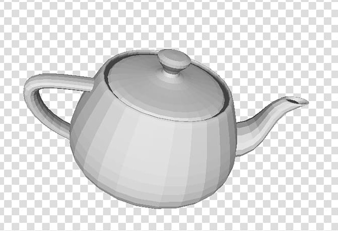
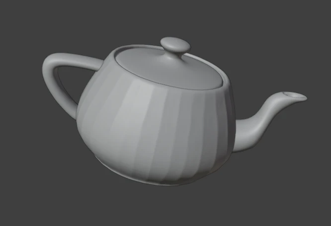
Simple object generation with Hunyuan v2.1 (Utah Teapot)
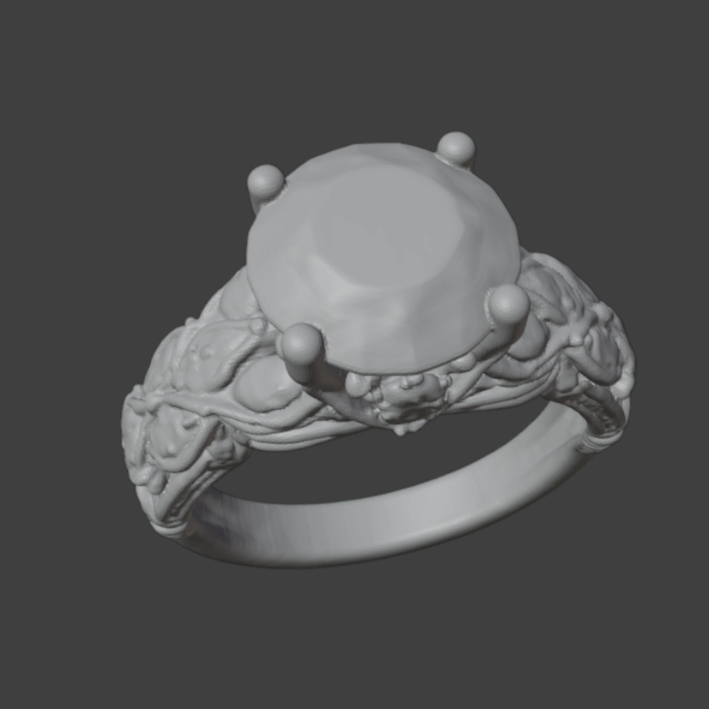
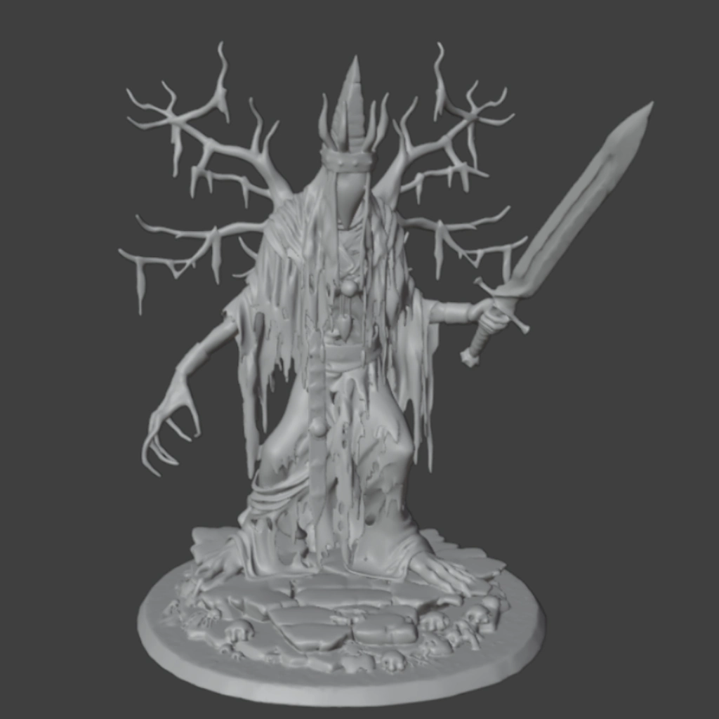
When we put standard shapes into these models, they come out nearly perfect, but such simple results barely provide additional value. The real test is where this technology meets industry-specific requirements, and currently, the winner is determined by how much “mess” your pipeline can tolerate. Advertising is the immediate sweet spot; since the goal is a beautiful view rather than perfect polygons, marketers can use heavy, unoptimized AI meshes for offline renders. E-commerce and entertainment sit in the middle, successfully using AI as a “prop factory” for rigid objects and background fillers where complex animation isn’t required. However, sectors such as gaming and high-end fashion remain the biggest laggards. Due to noisy topology and the absence of true physics simulation capabilities, AI still struggles to generate characters that deform correctly or dresses that realistically flow in the wind, leaving these areas stuck in a “prototype-only” phase until the next breakthrough. To back this up, let’s consider two industry examples: Video generation went through this same transition roughly two years earlier. For context on where 2D generation stands now, our AI video generation tools overview covers the current landscape; the trajectory in both fields is nearly identical.
EXAMPLE 1
EXAMPLE 2
INDUSTRY
Advertising/E-commerce
(Jewelry)
Manufacturing
(3D printing)
INPUT
A Gemstone Ring
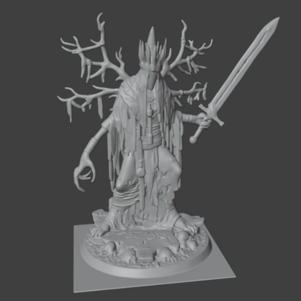
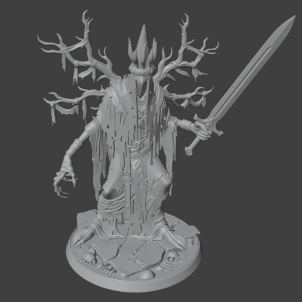
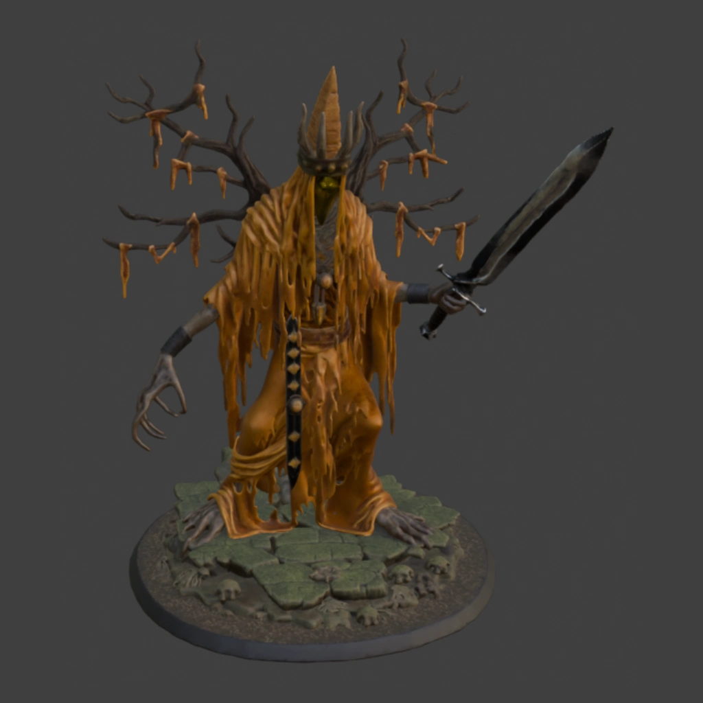
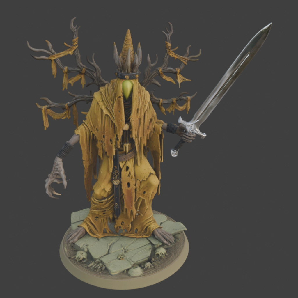
A Tabletop Monster Miniature
CHALLENGES
Requires sharp, hard-surface precision with reflective textures.
Features thin parts and a complex organic silhouette;
EXPECTED RESULT
Model that represents input image 1 to 1 without hallucinations, with smooth surfaces and geometrically correct gems.
The model has a distinct base, thin details represented well enough to be printable, and the whole mesh is watertight.
Advertising/E-commerce (Jewelry)
Input
Trellis v2
Hunyuan v2.1
Hunyuan v3.0
Manufacturing (3D printing)
Input
Trellis v2
Hunyuan v2.1
Hunyuan v3.0
At first glance, all models appear to perform well. There is an obvious dependency: the larger the model, the more satisfactory the results seem (and inference time increases). However, this raises the question of whether this trend truly holds.
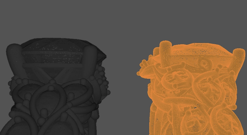
Hunyuan v3.0 (left) and Trellis 2 (Right) generations’ wireframes
Under a digital microscope, the wireframe’s clean surface dissolves into millions of chaotic triangles. When a human models a mesh, components like gems are built with minimal polygons and a logical structure, making minor edits as simple as moving a few vertices. You can also predict a skilled modeler’s quality based on their portfolio. Generative AI is different. Most algorithms extract meshes from latents with extremely high-density topology, making manual sculpting or editing a nightmare. It’s often faster to remodel the entire sample than to fix the topology by hand. Furthermore, performance is inconsistent; while models handle familiar shapes well, they often struggle with specific details or views, like Trellis with gems.
Trellis v2
Hunuan v3.0
Close-up of Hunyuan v3.0 textures
On to textures. While Hunyuan v3.0 wins on fidelity, Trellis v2 is better at keeping materials from bleeding into one another. However, both models struggle with PBR. Shadows and highlights are incorrectly painted onto the albedo rather than being handled by metalness and roughness channels. Because distinct materials are merged into a single layer, reusability and editing are nearly impossible. Often, what appears to be complex geometry is actually a “hallucinated” flat texture. For instance, Hunyuan v3.0 makes small diamonds look more like apricot seeds.
So, what are we left with?
The current state of 3D AI follows an 80-20 rule. For familiar objects and clean camera angles, you can expect nearly perfect results. However, that final 20% of accuracy is incredibly difficult to bridge. Unlike 2D AI, where you can easily use Photoshop or Inpainting, 3D models produce assets with such high-density, “messy” topology that turn polishing into a nightmare.
While all this may sound critical, the field has, in fact, skyrocketed recently. The leap from DreamFusion to models like Hunyuan v3 is massive, with new major breakthroughs still dropping every few months. We can get immense value from these tools right now, but they aren’t “plug and play.” They require specific tailoring, heavy post-processing, and cleanup to be production-ready. If you don’t think through your workflow, the costs for computing and polishing labor will add up quickly.
Custom AI 3D Generation Pipelines: How IT-JIM Builds Them
Turning raw AI output into a professional asset is where the actual engineering happens. You need a structured pipeline, which takes raw generations as “digital clay” and refines it into a production-ready geometry through five essential stages. The same mesh problems show up in device-based photogrammetry. Our 3D reconstruction on iOS guide covers the ObjectCapture workflow, which hits the same mesh density and topology walls described here.
The process begins with the first stage: Fine-tuning Generation. Since 3D models (TRELLIS, Hunyuan) are more temperamental than 2D tools like Stable Diffusion, you often need to adapt open-source models to your specific category or camera angles. This requires significant data and compute, as standard training scripts rarely run optimally (or correctly, in the case of Hunyuan) without heavy modification. In case anything goes wrong, as it often does with open-source code, pay attention to issues in the source repo. Even then, fine-tuning has limits and cannot fix every edge case. But it is almost always worth the effort as each step down the line depends on the quality of the initial generation.
The next stage is Segmentation, where you split a single, unmanageable mesh into components. Open-sourced models like P3-SAM, SAMesh, or PartField serve as the backbone here. Instead of fighting one massive blob, segmenting allows you to run specialized logic on different parts: fixing an important part with high fidelity while keeping the base as-is, or replacing it with some preset. This stage is the foundation for organized editing and material management, but it often takes more resources than the generation itself.
Because standard splitting often leaves “holes” where segments connect, Completion becomes the next vital stage, powered by models like X-part or HoloPart (both are open-source). This phase uses the initial mesh to “hallucinate” missing geometry, ensuring every segmented part is a separate, manifold object. This makes the assets physically viable rather than just visual shells, but comes at the cost of high memory requirements and additional time.
Texture Assignment follows as the next stage in the pipeline: AI textures made for the whole mesh can barely ever satisfy production. By having distinct geometry for different components, you can assign PBR materials from a high-quality database or run painting models on individual parts, ensuring that metal looks like metal and cloth looks like cloth.
Finally, the Cleanup stage addresses the chaotic topology. By using sequence-based tools like MeshAnything v2 that place vertices similar to a human artist, or applying remeshing algorithms to redistribute polygons, you can turn dense, uneditable topology into clean, even surfaces. It is far more reliable to retopologize these simple, segmented pieces than to attempt to fix a complex, branching mesh all at once.
The Current State of AI 3D Generation: Strengths, Limits, and What to Expect Next
Tracing the evolution of 3D AI from basic photogrammetry to sophisticated “Native 3D” models makes one thing clear: the technology has not yet achieved “out-of-the-box” usability for professional workflows. The gap between a chaotic AI hallucination and a production-ready asset cannot be bridged by simply waiting for a better model; it requires fine-tuning and the implementation of a robust post-generation workflow. This pipeline might involve segmenting the mesh into essential components, replacing parts with high-quality presets, or retopologizing for clean geometry. It may also require thickening thin parts to meet 3D printing requirements, assigning realistic PBR textures for a final render, or many other steps, depending on the specific use case.
While current technology excels at generating visual prototypes suitable for advertising and e-commerce, it still falls short of the rigorous topological and physical standards required for high-end manufacturing or gaming. In conclusion, we are not waiting for a model that does everything, but rather building the workflows that yield results here and now. As AI quality improves, it will open doors to previously unreachable industries. This progress creates a paradox: the better the models get, the more crucial the adaptation layer becomes to move from a simple visual prototype to a complex, physics-ready asset. If you are evaluating whether to build this kind of pipeline in-house or with a partner, our computer vision development services page covers how we work.
AI 3D Generation for Games, Jewelry, Fashion, and Advertising
The state of 3D AI plays out very differently depending on what you need to do with the output. In some industries the current models are good enough to ship; in others, a custom post-processing pipeline is the only thing that separates a prototype from a product.
Game studios
Game studios spend real money on environmental assets, props, and background characters that players rarely look at directly. AI 3D generation can already automate much of that work: rigid objects, furniture, vehicles. That frees artists for the characters and hero items that require real craft. The catch is topology: game engines want clean, low-poly meshes with proper UV maps, and raw AI output is neither. A post-generation pipeline that covers segmentation, retopology, and LOD generation turns that raw geometry into something a game engine can actually use. IT-JIM builds that kind of pipeline for studios that need to grow asset output without growing the team.
Jewelry and accessories retail
Jewelry e-commerce is a strong fit. Brands that add 3D and AR product views see higher conversion rates, and rings, pendants, and watches are exactly the rigid, hard-surface objects current models handle best. The problem is precision: gemstones and metallic settings require accurate PBR material separation that out-of-the-box models consistently get wrong. A pipeline fine-tuned on a brand’s own SKU catalog, paired with a curated material database for metals and stones, can produce render-ready assets at scale. The ring example from earlier in this article shows exactly what the starting point looks like. A custom pipeline is what closes that gap.
Fashion and apparel
Fashion is split. Anything that drapes or stretches still defeats current generation models. Rigid accessories (bags, shoes, eyewear) are a different story. A well-designed pipeline can triage SKUs by category: send accessories through the automated route and send garments to a 3D artist. That split alone cuts the cost per digital asset significantly.
Product visualization and advertising
Campaign renders only need to look right in a still image or short video. Nobody inspects the wireframe. AI-generated geometry, even with dense topology, is perfectly usable for offline rendering. A pipeline that goes from product photography to render-ready 3D asset is a practical, lower-cost alternative to commissioning a 3D modeler for each SKU.
Building production-ready 3D pipelines
The post-generation workflow in this article is real engineering work. Getting from a raw AI mesh to something production-ready requires expertise across computer vision, 3D geometry processing, and model fine-tuning. Clean topology, proper materials, and the right output format for your renderer or game engine do not come automatically. IT-JIM builds that pipeline for clients who need working output, not proof-of-concept demos.
We have fine-tuned open-source models like TRELLIS and Hunyuan on domain-specific data, built segmentation tools, and written retopology and material assignment steps that turn a dense AI mesh into something a game engine or e-commerce renderer can actually use. Several of those projects are in our portfolio.
If you are scoping out an AI 3D generation project in product visualization, game asset production, jewelry e-commerce, or another area and need a team that has already solved the post-generation side, get in touch.
If you’ve ever tapped on a person in an Instagram photo and watched them lift cleanly from the background as a sticker – that’s Meta’s Segment Anything Model working quietly behind the scenes. Instagram’s Cutouts feature, confirmed by Meta to be built on SAM, turned what used to be a careful manual masking job into a single tap. And with SAM 3, released in late 2025, the model took another step: it added text prompting. Instead of clicking, you can now type “yellow school bus” into a video and the model finds it, segments it, and tracks it through every frame. Now Meta has brought the same thinking to audio.
SAM Audio, released by Meta’s Superintelligence Labs in December 2025, does for sound what SAM did for images. Describe it, point to it in a video frame, or mark a moment in the timeline of a waveform where it’s clearly audible and the model separates it from everything else. One model covering tasks that previously each required their own specialized system: speech denoising, stem separation, speaker diarisation, instrument isolation, arbitrary sound extraction – the full range of audio processing services now addressable through a single promptable interface. As a foundation in multi-modal ai, it unifies text, vision, and temporal cues into a single generative system for sound. In this blog, we’ll walk through what the model can do, how well it actually performs in practice, and what the paper contributes to the audio AI field – including some details worth paying close attention to if you’re thinking about integrating or building on this technology.
Tell It What You Want: Three Ways to Talk to SAM Audio
The most natural way to think about SAM Audio is as a model with three different input channels, each suited to a different situation. They can be used independently or combined for more precise control.
Text prompt
The simplest starting point. You type what you want to extract. “acoustic guitar,” “crowd noise,” “male speech,” “violin section”, and the model does its best to find and isolate that sound within the mix. In practice, this turns the system into a powerful ai audio separation engine that behaves almost like a search bar for sound. This works well when the target is easy to describe and acoustically distinct from everything else around it. Think of it as a search bar for sound: most of the time, good enough phrasing gets you what you need. Where it starts to struggle is when the target is hard to pin in words, like close variants of similar sounds, for example, or a specific effect within a dense soundscape where text alone can’t fully disambiguate what you’re after. For similar-sounding targets coexisting in the same mix the video mask prompt is usually the handiest approach
Video mask
When there’s accompanying video, this prompting mode becomes genuinely powerful. Instead of describing the sound, you show the model where it’s coming from. Click on the drummer in the frame, draw around the guitar amplifier, tap on the speaker whose voice you want to isolate and the model extracts the audio associated with that visual region. For anyone working with video content, this replaces what would previously have required access to the original multitrack sessions. You just point. Although, for musicians searching for a particular sound effect, span prompting is where it gets most interesting and truly becomes an audio-native tool.
Span prompt
This is the most distinctive feature, and the one most worth understanding if you’re a sound engineer or producer. Instead of describing the sound or pointing to a visual source, you highlight a short segment of the audio timeline – a moment where the target sound is clearly audible and relatively isolated. That segment becomes a fingerprint. The model uses it to find and extract acoustically similar material throughout the rest of the recording. Think of a field recording where a specific bird call appears and disappears across a 10 min of material, or a backyard capture where you want to pull out just the sound of wind rattling a piece of metal, a texture you heard once clearly, buried somewhere in the mix. Find one clean moment where it’s audible, mark it, and the model hunts it across the whole track, isolating from residual sounds.
All three modes can be combined in any pair variation or be used independently.
How Good Does It Actually Sound?
This is the question that matters most for anyone considering using the model in a real workflow, and it deserves an honest answer rather than a recitation of benchmark numbers.
The first thing to understand is that SAM Audio is a generative model. It doesn’t carve a sound out of a mix the way a mask-prediction model would. It synthesizes a new version of the target sound, conditioned on the mixture and the prompt. This is an important distinction when it comes to evaluation. The standard objective metric for separation quality is SDR (Signal-to-Distortion Ratio), which works by comparing the model’s output sample-by-sample against a clean reference recording of the target sound. But since SAM Audio generates rather than extracts, even minor differences in timing between the output and the reference, things that are completely imperceptible to a human listener, cause SDR scores to drop. Comparing SAM Audio’s raw SDR numbers against those of a mask-based discriminative model is like comparing two different kinds of instruments on a scale calibrated for only one of them. The paper acknowledges this directly, which is part of why the authors developed new evaluation methods (more on that in the next section).
With that caveat in mind, across the benchmarks where comparison is meaningful (general sound separation, speech, music, and instrument separation in both in-the-wild and professionally produced recordings) – SAM Audio outperforms prior general-purpose models and reaches competitive or state-of-the-art performance against specialized systems that were purpose-built for a single domain. That’s a significant result: one model beating tools that were designed to do only one thing.
In real-world use, though, there’s a practical nuance worth knowing. The training data included not only high-quality studio recordings but also a large volume of medium-quality video audio, the kind of material you’d find on the internet, recorded with phone microphones in noisy environments. This is actually what gives the model its broad generalization ability. But it also means the model has learned many sounds as they typically exist in the wild: embedded in their natural context, surrounded by ambient noise. When you try to isolate something like an ambulance siren, or the sound of a passing train, or distant crowd noise (sounds that in real recordings almost never appear in silence) – you’ll often find that the extracted result carries some of that environmental texture with it. The model isn’t doing something wrong; it’s producing what it learned is a realistic version of how that sound exists in the world. It’s something to factor in when choosing whether SAM Audio is the right tool for a given task, versus a more specialized model trained on cleaner data for a specific domain.
Under the Hood. What the Paper Actually Contributes
From here, we’re getting more technical. This section is aimed primarily at deep learning engineers and researchers. The paper makes contributions in four areas worth looking at closely: the generative architecture, span prompting, a new automatic evaluation model, and a new approach to subjective evaluation.
Architecture
SAM Audio is built on a Diffusion Transformer trained with flow matching. The core framing is important: the source audio mixture is not the direct input being processed – it’s a conditioning signal. The model learns to generate the target stem by iteratively refining from noise, guided jointly by the audio mixture and the user’s prompt. This is fundamentally different from the mask-prediction paradigm that has dominated audio separation (Demucs, MossFormer2, and most production-grade separation tools fall into this category). Those models effectively learn a filter: given the mixture, predict a mask that when applied recovers the target. SAM Audio doesn’t filter – it generates. The architecture is much closer to how modern music or image generation models work, where the source material conditions the generation process rather than being directly transformed. Prompt encodings – text via a language encoder, video via visual features from masked regions, spans by tokens aligned to audio frames – are all injected as conditioning into the Diffusion Transformer alongside the mixture representation.
Span prompting
Technically, span conditioning works by converting the selected time intervals into a frame-synchronous binary token sequence. Each frame is marked as either silent (<sil>) or active (+) depending on whether the target event is present. This sequence is embedded via a learnable embedding table and concatenated channel-wise with the audio features before entering the DiT backbone, giving the model an explicit temporal prior about when to extract rather than what the sound is. This is fundamentally different from reference-based speaker extraction methods, which require a clean enrollment recording of the target source. SAM Audio needs only a timestamp.
One particularly useful implementation detail from the paper: when a user provides only a text prompt, it can use a secondary model called PEA-Frame that automatically predicts the frame-level activity of that sound event within the mixture and feeds it back as span conditioning. The paper shows that joint text + span conditioning consistently outperforms text-only prompting, so when you describe a sound in words, the model can quietly upgrade itself to also know when that sound is happening.
SAM Audio Judge (SAJ)
Evaluating GENERATIVE separation models is genuinely hard. SDR requires a clean reference, which doesn’t exist for real-world recordings, and is also biased against generative outputs for the timing reasons described above. CLAP similarity – another reference-free metric that measures how well the output matches the text description in an embedding space – turns out to correlate poorly with actual human judgment of separation quality, as the paper demonstrates. SAJ is a model trained directly on human perceptual quality annotations. It takes a mixture, text prompt and a separated output and predicts a quality score without needing a reference, and its predictions correlate much more strongly with human listening test results than CLAP similarity does. This matters well beyond SAM Audio itself – SAJ is a genuinely useful contribution to anyone working on audio separation evaluation, providing a way to assess real-world separation quality without the constraints of synthetic benchmarks.
Subjective evaluation protocol
The paper also rethinks how listening tests are designed for this class of model. This is a harder problem than it looks, and the paper redesigns the evaluation protocol from scratch rather than reaching for the standard tools.
MUSHRA (the traditional approach) requires a clean reference stem to compare against, which simply doesn’t exist for real in-the-wild recordings. Single-stimulus MOS tests avoid that dependency but are poorly sensitive to small differences between models and prone to anchoring drift across a session. The paper sidesteps both with a side-by-side Absolute Category Rating protocol with an always-on preference tie-breaker. Listeners see two model outputs for the same input alongside the original mixture and prompt, scoring each independently across three dimensions: Recall (how much target made it into the extraction), Precision (how much non-target leaked in), and Faithfulness (how similar the extracted sound is to the original mix). They then answer a forced-choice preference question regardless of whether their numerical scores already differ. The SAJ model described earlier was trained to predict these exact human scores – which is why it correlates so much more strongly with listener judgment than SDR or CLAP similarity. The subjective protocol isn’t just a validation step; it’s the foundation the automatic metric was built on.
Taken together, the target sound separation field has been dominated by discriminative, mask-predicting models. SAM Audio is a fully generative pipeline end-to-end – the first foundation model of this kind that unifies text, visual, and temporal span prompting in a single framework, and that matches or exceeds specialized systems across multiple domains simultaneously.
Conclusions
SAM Audio is a meaningful step for the audio AI field as a genuine foundation model that consolidates tasks previously requiring separate specialized systems into one flexible, promptable interface, covering speech, music, and general sound.
The real excitement, though, is what comes next. A model like this is a building block. It enables agents that can understand audio contextually and respond to natural language instructions – a mix engineer describing what they want rather than reaching for a plugin, a post-production workflow that can process field recordings based on spoken instructions, a creative tool for musicians that lets them explore separation as part of composition. The combination of span prompting with generative quality opens up use cases that simply weren’t possible before.
If you’re also evaluating the generation side of the same 2026 open-source wave — which models produce full songs from lyrics or prompts, how they license, and which are actually ready to build on — our open-source music generation model comparison covers eight models tested head-to-head.
Human pose estimation has emerged as a cornerstone technology in next-gen fitness and video analysis applications. For sports startups and developers building AI-powered coaching or performance tracking apps, real-time posture and movement analysis unlocks new value far beyond step counters or GPS tracking. Pose estimation is becoming foundational in AI-powered sports training where real-time feedback and motion tracking outperform legacy wearables.
Among available pose estimation frameworks, Google’s MediaPipe stands out as a popular choice for mobile-first MVPs. It’s fast, lightweight, and surprisingly production-ready but it also comes with its own quirks and architectural trade-offs. This article explores:
Why MediaPipe is often chosen for sports AI prototypes
How it compares to alternatives like OpenPose, ARKit Vision, and MoveNet
Common pitfalls when deploying MediaPipe on iOS and beyond
How to turn raw pose data into actionable video analysis and performance insights
Why MediaPipe Is a Go-To for Sports MVPs
MediaPipe is more than a pose estimation model. It’s a graph-based perception framework optimized for real-time mobile video analysis pipelines. Sports app developers choose MediaPipe for its:
Fast experimentation loop: Python prototype to mobile integration in days
Out-of-the-box pipelines: Pose, hands, face, and holistic models ready to deploy
Efficient on mobile: Runs on CPU or GPU with low latency (30+ FPS on mid-range phones)
On-device privacy: Enables edge-based video analysis without cloud compute
That said, MediaPipe only provides raw pose estimation landmarks. To deliver sports-specific insights, developers must implement domain logic like biomechanical metrics, rep counting, and performance scoring.
What MediaPipe Enables in Sports Apps
Posture and alignment feedback through pose estimation
Phase segmentation (e.g. analyzing stages of a golf swing)
Timing, symmetry, and video analysis for athlete movement
What MediaPipe Doesn’t Do Natively
Detect or interpret equipment (e.g. racket, club, bat)
Deliver actionable coaching feedback out of the box
Provide sports semantics – those must be manually built
Pose vs Holistic Models
Pose model: Easier to integrate, supports multiple people, but can misidentify limbs
Holistic model: More stable anatomically, includes face and hands, but single-person only
Framework Comparison: MediaPipe vs OpenPose vs ARKit vs MoveNet
Feature
MediaPipe (BlazePose)
OpenPose
Apple Vision Framework
MoveNet
Platform Support
Android, iOS, Web, Desktop
Cross-platform (GPU required)
iOS only
Android, iOS, Web
Performance
Real-time (30+ FPS)
GPU-dependent, slower
60 FPS on iPhones
Real-time mobile
Accuracy & Keypoints
33 landmarks
25+ landmarks
19 joints
17 landmarks
Multi-Person Tracking
Limited
Excellent
Single person
Single person
3D Depth Capability
2.5D relative depth
Mostly 2D
Full 3D if LiDAR
2D only
Ease of Integration
Easy for basics; harder for custom pipelines
Complex; research-focused
Seamless for iOS only
Developer-friendly
Tech Pitfalls: Limitations of MediaPipe in Sports Video Analysis
While MediaPipe performs impressively in ideal conditions, developers should be aware of its limitations in real-world sports contexts:
Model Accuracy and Depth
BlazePose is not anatomically constrained
Depth estimates can be unstable or noisy
2D overlays look clean but don’t translate well to biomechanics
Limb orientation may flip (e.g. arm facing camera vs away), which breaks 3D interpretation
Multi-Person and Occlusion Challenges
Holistic model only tracks one person
Pose model handles multiple users but can randomly flip limbs direction if they point towards or away from camera
Hands may appear disconnected or incorrectly matched when athletes overlap
Extra limbs or partial hands in frame cause rapid degradation; If three hands are visible – expect failure
Sports-Specific Edge Cases
Detection range is limited for distant players (e.g. on a tennis court)
Equipment (rackets, clubs, bats) often confuse the model
Two close hands holding a device may appear unrealistically far apart in 3D, which indicates underrepresentation of such cases in training data
Side angles or fast spins reduce tracking fidelity
Eye and Face Tracking
Assumes symmetrical eye movement
Model may mirror or misinterpret one eye
Uneven gaze tracking due to dataset imbalance
For developers working on face-centered features like eye state or attention detection, Apple’s native Vision Framework offers an alternative with better depth and stability in iOS-only contexts.
These gaps are why advanced sports and healthcare apps often evolve past MediaPipe’s stock models.
From Pose Estimation to Sports Insights
Landmarks alone don’t deliver value. A production-grade video analysis or fitness AI solution needs:
Pose retargeting to compare against an ideal motion pattern
MediaPipe offers great signal quality, but interpretation still happens downstream. Turning that signal into a sports product requires domain expertise and product design.
Techniques adapted for athlete motion have also proven effective in assessing motor symptoms during neurological movement analysis.
Deploying MediaPipe to iOS and Other Platforms
MediaPipe’s cross-platform promise includes iOS, Android, web, and desktop. But iOS presents specific technical challenges:
Uses Bazel for builds, not CocoaPods or SwiftPM
Requires building custom frameworks in C++
Real-time runs at ~30 FPS, but UX suffers without smoothing and gating logic
Still, the benefits are compelling: no cloud, fast on-device pose estimation, and strong privacy compliance. Developers experimenting with MediaPipe’s native API can explore a minimal working example in this C++ starter tutorial.
For Android, MediaPipe is available via Gradle or precompiled AARs. On the web, MediaPipe.js runs directly in-browser using WebAssembly, making lightweight video analysis available with no installation.
Signs You’ve Outgrown MediaPipe
When do you need something beyond MediaPipe?
Multi-person tracking must be stable and identity-aware
Precision is essential for clinical or rehabilitation use
Building sports apps that can handle real-world edge cases, from occlusion to equipment interference, often requires more than off-the-shelf tools.
Conclusion
MediaPipe is a flexible, efficient, and surprisingly powerful tool for real-time pose estimation and video analysis in sports and fitness apps. Its unique architecture and mobile-first design make it ideal for MVPs and on-device intelligence. But successful deployment requires more than plugging in a model. You’ll need to:
Build post-processing for stability and interpretability
Design your analytics pipeline for real-world edge cases
Understand when MediaPipe is sufficient and when it’s time to go custom
For companies scaling beyond MVPs, we help deliver robust sports ai solutions that translate motion into measurable outcomes.
Wearable fitness trackers and smartwatches have become standard gear for athletes, collecting metrics like heart rate, speed, and distance. However, these devices often fail to provide insights into how the movement was performed. Enter pose estimation, a computer vision technique that extracts biomechanical data from video, opening up new frontiers in sports performance tracking, sports analytics, and sports analytics software.
From What to How: The Shift Toward Movement Understanding
Traditional tracking answers “what happened” such as steps taken, GPS distance, or calories burned. But high-performance training and injury prevention demand deeper insights into how the athlete moved. Pose estimation enables that by analyzing joint angles, symmetry, sequencing, and compensation patterns, offering new capabilities in sports analytics and sports analytics software.
Using just smartphone video, pose estimation software can turn visual input into a detailed map of joint movement without expensive motion capture labs. This opens up scalable applications in sports performance tracking, enabling remote coaching, video analysis, and rehab monitoring.
Why Pose Estimation Matters for Sports Training
Pose-based video analysis enables:
Detailed Technique Analysis Coaches can see exactly how an athlete moves, such as knee angle during squats, arm swing symmetry, and hip extension. This enables targeted feedback and performance optimization.
Injury Risk Detection Pose tracking flags risky mechanics such as valgus knee movement and asymmetries that often precede injuries. This is critical for both elite athletes and youth programs.
Personalized Coaching and Rehab Training programs can be tailored to individual biomechanics. In rehab, pose-based tracking ensures symmetry and progress through recovery.
Progress You Can See Improvements in sprint angles, stroke straightness, or jump technique can be quantified and tracked over time, motivating athletes to train smarter, not just harder.
Remote and Scalable Coaching Athletes can record practice on their phone, receive pose-driven feedback, and compare their form to elite models without requiring an in-person session.
Pose estimation complements wearables. Together, they deliver a 360-degree view of athlete performance.
Core Features of a Sports Performance Tracking App
Let’s break down what goes into a successful sports analytics software solution.
Key Features
Video Capture and Upload Easy-to-use camera interface with guidance for framing athletic movement.
Pose Estimation and Metrics Extraction AI analyzes frames for biomechanical data such as knee angles, stride symmetry, and joint velocities.
Visualization and Feedback Skeleton overlays, comparison videos, angle charts, and coach-style feedback like “Your landing angle is 12 degrees below optimal.”
Session History and Tracking Progress tracking over time is ideal for athletes and coaches measuring training impact.
Multi-Athlete Coaching Interfaces For teams or training platforms, coach dashboards allow reviewing, commenting, and planning across users.
Tech Stack Considerations
Pose Estimation Engine MediaPipe is a popular choice for MVPs thanks to efficient on-device inference.
Mobile App Development Native iOS and Android apps offer tight performance, but cross-platform tools like Flutter or React Native are also viable depending on the team.
Backend Infrastructure Cloud services such as Firebase support user management, video uploads, and session history. For heavier analysis or multi-angle processing, cloud-based inference pipelines using GPUs can be deployed alongside mobile apps.
Post-Processing Logic Jitter filtering, confidence gating, and biomechanics-driven insights are essential for user trust.
Front-End Visualization Clean, intuitive UI for displaying movement metrics, skeleton overlays, and progress graphs is key to user adoption.
What Strong Apps Do Differently in Sports Analytics
Apps that succeed in the market tend to:
Prioritize post-processing and biomechanics, not just raw pose data.
Handle real-world camera variability including occlusion, angles, equipment, and lighting conditions gracefully.
Top developers understand that pose detection is infrastructure. The real value lies in the insight layer built on top.
Strategy: From MVP to Custom Models
A smart development path:
Start with MediaPipe to validate product-market fit.
Test real-world video conditions such as occlusion, body type variance, and sports equipment.
Replace components as needed with custom-trained models or cloud inference once requirements mature.
Out-of-the-box tools like MediaPipe work best for:
Single subject in frame
Controlled camera distance and angle
Minimal occlusion
They struggle with:
Sports involving gear such as bats or rackets
Partial-body or first-person inputs
Medical-grade accuracy or neuro assessments
When you’re ready to scale beyond MVP, consult our MediaPipe Tech Review to understand performance trade-offs.
Choosing the Right Sports App Development Company
If you’re planning to build a next-generation sports analytics software app, choose a sports app development company with:
Mobile deployment expertise with strong performance on iOS
Computer vision and machine learning capabilities
A track record converting noisy pose data into clean, actionable feedback
Whether your application demands lightweight edge processing on mobile or high-fidelity, multi-angle analysis in the cloud, your development partner should be equipped to handle both extremes.
The biggest challenge is not pose detection but creating consistent, trusted insights from variable video environments. That is why domain expertise and real-world UX testing are essential.
To explore our solutions, check out our full offering on the Sports Industry Page.
Final Thoughts
Pose estimation shifts the focus from activity tracking to true movement understanding. For startups, coaches, and sports tech brands, it enables scalable coaching, personalized feedback, and smarter training apps.
Whether you’re launching a niche product or building the next big coaching platform, combining pose estimation with biomechanics intelligence and mobile UX is your ticket to standing out.
Now is the time for fitness innovators and sports app developers to move beyond smartwatches and into the era of AI-enhanced sports performance tracking.
In 2020, Billie Eilish swept the Grammys: Album of the Year, Record of the Year, Song of the Year, Best New Artist. The album that won it all was recorded in her brother’s childhood bedroom on a setup that cost less than $3,000. Accepting the award, producer Finneas dedicated it to “all the kids making music in your bedroom.”
A decade earlier, this would have been unthinkable. For most of recording history, making a professional record meant booking expensive studio time, hiring engineers, and accessing gear that cost more than a house. Digital audio workstations changed that. Today, a laptop and a $200 microphone can produce Grammy-winning music.
Beyond cost, something bigger shifted: who gets to create. And every step of the way, skeptics asked the same questions: Is this real music? Is this cheating? Will this replace real artists? Now, AI is the next wave. And the questions sound exactly the same.
This shift is now being accelerated by AI music technology, as a new generation of AI-powered music tools becomes part of everyday creative workflows for musicians.
The AI Music Landscape in 2025
The change is already happening. In 2025, Deezer disclosed that over 20,000 AI-generated tracks were uploaded to its platform daily, representing 18% of all uploads. Suno, the leading AI music platform, has reached nearly 100 million users and raised $250 million at a $2.45 billion valuation. Major labels are taking notice: Warner Music Group settled its copyright lawsuit with Suno and entered a licensing deal, signaling a shift from resistance to collaboration.
But so far, the more interesting story seems to be how AI is becoming part of the creative workflow, not replacing it. Suno’s latest product, Suno Studio, illustrates this perfectly. Described as the world’s first generative audio workstation, it blends generative features with professional multi-track audio editing. Musicians can upload samples, edit in a multitrack timeline, control BPM, volume, and pitch, generate unlimited stem variations: vocals, drums, synths, and export everything as audio and MIDI to continue working in their existing DAW. As Suno’s CEO put it: “Studio was built to expand the toolkit for musicians; it intentionally does not prescribe workflows so that human talent can remain front and center.” This reflects a broader trend in AI music processing, where tools are designed to augment human creativity rather than automate it away.
A recent survey of 1,200 music creators found that 87% of artists have incorporated AI into at least one part of their process from songwriting and production to promotion. The ability to fill skill gaps is the most celebrated benefit of AI, driving the rise of self-sufficient creators who can handle every stage of their release cycle. These results highlight how quickly AI tools for musicians are becoming a standard part of modern music production.
In this blog, we’ll review some of the most interesting AI products and open-source models that are extending the possibilities of how artists create music – tools that enhance creativity, without replacing it. Fair warning: some of these products are pretty specialized, and explaining audio tools in text has its limits.
Music AI Products that Extend the Artist’s Toolkit
Synplant 2: Creating Truly New Sounds with Neural Networks
One common criticism of generative AI is its perceived lack of originality. And it actually makes sense: generative models learn the underlying probability distribution of their training data and optimize to sample from that distribution given a prompt. In music generation, this means outputs often recombine existing patterns instead of creating something fundamentally new.
Creating truly new sounds has traditionally required significant effort: hours spent tweaking synthesizer parameters, recording and processing real-world audio, or experimenting with unconventional techniques. Synplant 2, developed by Sonic Charge, offers a different approach that uses neural networks not to generate music, but to accelerate the discovery of new timbres.
At its core, Synplant 2 is a two-operator FM synthesizer with a unique “genetic” interface. The main feature is Genopatch: a machine learning system trained not on existing music, but on the synthesizer engine itself. The neural network learns the inverse mapping – from sound back to parameters – so when you feed it any audio recording, it makes educated guesses about which settings would produce a similar result.
The output from Genopatch is a playable synth patch, not just an audio clip. Each generated patch becomes a starting point for further exploration through Synplant’s mutation system or DNA Editor. This makes Synplant 2 a strong example of AI music technology focused on sound design rather than composition.
Project LYDIA: New Ways to Interact with Sound
Another compelling example of AI opening new possibilities for instrument interaction is Project LYDIA, a collaboration between Roland Future Design Lab and Tokyo-based AI studio Neutone, announced in November 2025. Project LYDIA demonstrates how audio AI and machine learning can redefine how musicians interact with instruments in real time.
Project LYDIA, named as a nod to both “DIY” and “AI” – is a hardware prototype built on a Raspberry Pi 5 that brings Neutone’s Morpho technology into a compact, stage-ready pedal format. The core concept is what Neutone calls “neural sampling”: using an autoencoder neural network to learn the tonal characteristics of any sound source, then applying those characteristics to incoming audio in real time.
The technology works by training a model on a collection of sounds – this could be a traditional instrument like a violin, but also field recordings, environmental textures, or any audio you can capture. The neural network learns a compressed representation of how those sounds behave: their frequency content, how harmonics rise and fall, their overall timbral fingerprint. Once trained, you can feed any live input (your voice, a guitar, a synthesizer) through the model, and it will reshape that input to carry the timbral qualities of the training material while preserving your original pitch, dynamics, and articulation.
What makes Project LYDIA interesting is the shift in how musicians can interact with sound. Traditional effects process audio through fixed algorithms; samplers trigger pre-recorded material. Neural sampling does something different: it lets you play through a learned understanding of sound. You’re not triggering a recording of a djembe – you’re transforming your input through what the model has learned about how djembes sound. The result is something that responds to your playing in real time while inhabiting a completely different sonic space.
This approach also removes the traditional boundaries of what can become an “instrument.” Users can train models on sounds that were never meant to be musical – the texture of a busy street, the hum of machinery, the ambiance of a specific location, and perform with them on stage. The choice of training material becomes a creative decision in itself.
ACE Studio AI Violin: Beyond the Limitations of Sampling
Speaking of moving beyond discrete sample triggering – ACE Studio’s AI Violin, released in beta in May 2025, applies a similar principle to virtual instruments.
Traditional digital music production relies heavily on sampling: large libraries of pre-recorded instrument performances triggered by MIDI data. A violin sample library might contain hundreds of gigabytes of recordings of different notes, articulations, dynamics, and bowing techniques all stitched together when you play. The challenge is that real musical performance is continuous and deeply contextual. A violinist doesn’t think in discrete samples; they shape phrases, transition between notes, and apply expression in ways that are difficult to replicate by sequencing isolated recordings. Making sampled instruments sound natural requires significant skill: programming keyswitches, drawing expression curves, and manually compensating for the inherent discontinuities between samples.
ACE Studio’s AI Violin takes a different approach. Instead of triggering pre-recorded samples, it uses machine learning to synthesize performances directly from MIDI input. The neural network has learned the characteristics of violin performance: bowing, vibrato, dynamics, tonal color, phrasing; and generates audio that exhibits these qualities in context. You input a melody, and the AI produces a performance with natural transitions, appropriate articulation, and expressive nuance, without requiring the producer to manually program every detail. It represents a new class of AI-powered music production tools that move beyond traditional sampling.
BIAS X: Recreating Any Guitar Tone in Seconds
Beyond creative possibilities, AI can also save significant time in the practice and production workflow. Consider the process of practicing electric guitar. Part of mastering a song involves dialing in the right tone, the specific combination of amp settings, effects, and cabinet characteristics that define how the guitar sounds. When you want to play along with a particular track, recreating that exact tone traditionally requires hours of tweaking: adjusting gain staging, experimenting with EQ curves, layering effects, and comparing against the reference. For many players, this technical overhead becomes a barrier to simply playing.
BIAS X, released by Positive Grid in September 2025, addresses this directly with AI-powered tone matching. The software offers two approaches: “Text-to-Tone” lets you describe the sound you’re after in natural language , like “creamy blues lead with a hint of delay” or “90s Swedish death metal rhythm”, and the AI builds a complete signal chain. “Music-to-Tone” goes further: drop in a guitar track or full song, and BIAS X analyzes the tonal characteristics and reconstructs a matching preset. This is a practical example of AI music processing reducing technical friction in everyday creative workflows.
The system was trained on over one million tones and analyzed more than 200 amplifiers to understand the nuances of genre, era, and playing technique. When you upload a reference, it examines spectral and dynamic profiles to approximate the amp, cabinet, and effects chain. The result isn’t always a perfect one-to-one match, but it provides an excellent starting point from which you can refine it either conversationally, asking for “more bite,” “less reverb,” or “tighter low end” or using parameters directly.
This represents a shift in how guitarists interact with their sound. Instead of translating a tonal idea into technical specifications like “I need a mid-scooped high-gain amp with a tube screamer in front and a plate reverb”, you can simply describe what you hear in your head or point to an example. The AI handles the translation, letting you focus on playing.
Open-Source AI Music Technology and Models for Music Creation
Beyond commercial products, a thriving ecosystem of open-source models has emerged, giving musicians and developers access to state-of-the-art deep learning architectures and ability to customize further. These projects often push the boundaries of what’s technically possible, and many commercial tools build on or are inspired by this open research.
Demucs: Stems for Everyone
Ever wanted to isolate the bassline from a track to learn it by ear? Or pull out vocals for a remix? Stem separation (splitting a mixed song into its individual parts) used to require access to the original recording sessions. Demucs, developed by Meta AI Research, changed that by making high-quality separation available to anyone. It has become a foundational audio AI model for music source separation.
Drop in a song, and Demucs splits it into vocals, drums, bass, and everything else. The results are clean enough that musicians actually use them, not just as a curiosity, but as part of their workflow. Producers sample isolated elements into new tracks. Guitarists mute the original guitar to practice over the rest of the band. DJs create acapellas and instrumentals on the fly. Teachers extract individual parts for students to study.
What makes Demucs different from earlier separation tools is that it works directly on the audio waveform rather than on spectrograms. Without getting too deep into the technical weeds: this approach preserves more detail and produces fewer of those watery, artificial artifacts that plagued older methods.
There are plenty of commercial stem separators now, many built on similar technology, but Demucs remains a go-to for anyone who wants a free, open-source option they can run locally and customize. For developers and researchers, it’s become the baseline that everyone else measures against.
For more structured music tasks like AI music transcription, newer architectures such as Mamba are enabling faster and more accurate piano transcription systems.
RVC v2: The Voice Conversion That Went Viral
If you’ve stumbled across a YouTube video of Frank Sinatra singing “Blinding Lights” or SpongeBob performing death metal, you’ve heard RVC in action. Retrieval-based Voice Conversion took the internet by storm with AI covers, some hilarious, some eerily convincing, and introduced millions of people to what AI could do with music. RVC illustrates how accessible music AI models can rapidly shape creative culture.
But behind the memes, RVC is a genuinely useful tool. It takes a voice recording and transforms it to sound like someone else while keeping the original timing, phrasing, and emotion intact. Think of it as a real-time voice skin: you sing, and the output sounds like the target voice.
The creative applications go well beyond novelty covers. Artists can produce songs in languages they don’t speak by hiring a native singer to perform the vocals, then use voice conversion to transform it into their own voice. Solo producers can create male-female duets without hiring a second vocalist. Some musicians have even trained RVC on instrument samples instead of voices, with which you can sing a melody, and it comes out as a saxophone or violin, useful for sketching ideas quickly.
What made RVC v2 particularly significant was accessibility. The model can be fine-tuned on as little as 10 minutes of clean audio, meaning anyone with a decent microphone and some patience can create a custom voice model. This low barrier helped RVC become the most widely-used voice conversion tool in the open-source community – the baseline that newer models are still compared against.
There are more advanced commercial alternatives now, but RVC’s popularity and community support keep it relevant. For many musicians experimenting with voice conversion for the first time, it’s still the starting point.
ACE-Step: A Foundation Model for Song Generation
The music generation tools that grabbed headlines – Suno, Udio, didn’t emerge from nowhere. They built on years of open-source research, with models like Meta’s MusicGen and Stability AI’s Stable Audio pushing the technology forward in public. For anyone wanting to experiment with music generation these open models have been essential.
The current open-source state-of-the-art for full song generation with vocals is ACE-Step, developed jointly by ACE Studio and StepFun. Think of it as the Stable Diffusion of music: a foundation model designed to be flexible, fast, and customizable. ACE-Step represents a new generation of generative music AI built as a flexible foundation model.
What sets ACE-Step apart technically is its diffusion-based architecture. Without diving too deep: this makes it significantly faster than models that generate audio token-by-token. It can produce up to 4 minutes of music in roughly 20 seconds on professional hardware.
But speed isn’t the main appeal. Because it’s diffusion-based, ACE-Step supports features that sequential models struggle with: inpainting (regenerating just a section of a song while keeping the rest), remixing existing audio, and using your own content to influence generations. So it’s not only for “type a prompt, get a song” – artists can feed in their own material and shape the output.
For those wanting to go further, ACE-Step supports LoRA fine-tuning. In plain terms: you can train a lightweight adaptation of the model on your own music, so generations come out closer to your style without needing massive computing resources or starting from scratch.
Released under an open Apache 2.0 license with support for 19 languages, ACE-Step gives independent developers and musicians a foundation to build on. It won’t match the polish of commercial products yet, but it’s where a lot of experimentation is happening. If you want to see exactly where ACE-Step 1.5 lands relative to the other models that shipped in 2026 — LeVo 2, Khala, DiffRhythm 2, and four others — we ran a head-to-head listening test across all of them and wrote up the results, including what each license actually permits
SAM Audio: Point at a Sound and Isolate It
We already covered Demucs, which splits music into fixed categories: vocals, drums, bass, and the rest. SAM Audio, released by Meta in December 2025, takes separation much further: it isolates whatever sound you ask for. This kind of targeted extraction is an emerging capability in advanced audio AI systems.
Want just the violin from an orchestral recording? Type “violin” and it pulls it out. Working with video and need to isolate a specific sound effect? Click on the object in the frame making the sound. Have a section of audio where the target sound is clear? Mark that segment as a reference, and the model finds and extracts similar sounds throughout the mix.
This flexibility with text prompts, time-range references, or even clicking on objects in video opens up new possibilities for sampling and sound design. Grab a specific percussion hit buried in a complex mix. Isolate a texture you like from someone else’s track to study how it was made. Extract a sound from a video clip to build a custom sample library.
The technology builds on Meta’s “Segment Anything” approach from computer vision, adapted for audio. It runs faster than real-time, so you’re not waiting around for results.
Demucs remains the go-to for straightforward stem separation. SAM Audio is for when you need something more specific – when the predefined categories aren’t enough and you know exactly what you’re after.
Many of these approaches extend beyond music into audio AI services, including speech, voice, and general sound processing.
The Toolkit Keeps Growing
The products and models in this post are just a snapshot, a few interesting cases that show how AI tools for musicians are evolving. This field moves fast, and there’s certainly more impressive stuff on the horizon. Together, these tools illustrate how rapidly AI music technology and audio AI services are evolving. For a current snapshot of where open-source song generation actually stands — eight models, three genres, license-by-license — our study covers the full picture.
This overview is not exhaustive. It focuses on tools that enhance musicians’ capabilities rather than replace their strengths. Seeing AI positioned as a creative partner, not a substitute, is what makes this space particularly compelling.
Want to shape this future too? If you have an idea for a music AI tool and need a team to bring it to life, we’d love to hear from you. Our AI music services for the music industry page outlines the kinds of systems we help teams build – from creative tools to production-ready music AI solutions.
Have a project you’d like to discuss? Contact us below or reach out at hello@it-jim.com.
AI music technology is becoming a critical layer in modern digital products. Music education platforms, creative software, rights management systems, and large-scale media services increasingly rely on accurate and fast transcription to unlock value from audio data.
In our work with AI music processing systems, we see that traditional transformer-based approaches, while accurate, are often expensive to operate and difficult to scale. This article outlines how Mamba, a selective state-space model architecture, enables high-performance, cost-efficient AI music technology suitable for real-time and production environments. Hands-on research and experimentation behind this work was done by Roman Bernikov, who focused on model architecture choices, evaluation methodology, and performance optimization.
AI Music Technology Use Cases and Business Impact
Efficient transcription underpins many real-world AI music technology products, including:
Real-time music education and performance feedback
Large-scale music catalog indexing and analytics
Creative AI tools and digital audio workstations
Edge and on-device AI music technology
Enterprise-scale batch music processing
These are representative of the AI music processing challenges encountered in production audio AI services.
The Scalability Challenge in AI Music Technology
Automatic Music Transcription (AMT) converts raw audio into symbolic representations such as MIDI or piano rolls. Transformer-based models dominate benchmarks but scale poorly with sequence length, leading to increased latency and infrastructure cost.
In production audio AI services, this directly impacts feasibility for long recordings, real-time interaction, and cost-efficient deployment.
Why Mamba Is a Strong Fit for AI Music Technology
Mamba is a selective State Space Model (SSM) designed for linear-time sequence processing. Rather than relying on attention across all time steps, it maintains a learned internal state that evolves dynamically with incoming audio frames.
From a deployment perspective, this provides:
Linear inference time
Stable memory consumption
Efficient GPU execution
These characteristics are especially valuable when building scalable audio AI services.
Designing a Production-Oriented AI Music Transcription System
The transcription system follows a design approach we commonly apply in client projects:
Spectrogram-based feature extraction
Lightweight convolutional preprocessing
Efficient long-range sequence modeling using Mamba
Task-specific prediction heads
While more complex variants were explored, a unidirectional Mamba architecture with skip connections delivered the most reliable balance between accuracy, simplicity, and inference efficiency, which are key requirements for production systems.
Accuracy Evaluation
System outputs were evaluated against ground truth MIDI annotations from the MAESTRO dataset. Metrics included onset timing, offset accuracy, frame-level alignment, and velocity estimation.
The model consistently captured musical structure and timing, with most errors occurring in ambiguous regions such as soft notes or dense passages. While absolute benchmark scores did not exceed heavily optimized transformer models, performance was competitive given the significantly simpler architecture.
For client-facing AI services, this level of consistency and predictability is often more valuable than marginal benchmark gains.
Efficiency Gains That Enable Scalable AI Music Technology
Inference benchmarks show that the Mamba-based system transcribed 30 minutes of audio in approximately 1.3 seconds, an order-of-magnitude improvement over transformer-based approaches and an impressive 1300 faster than realtime .
In production AI services, these gains translate directly into higher throughput, lower cloud costs, and the ability to support real-time user experiences.
Conclusion
Mamba-based architectures enable a shift toward deployable, efficient AI music technology. By combining competitive transcription quality with exceptional inference efficiency, this approach aligns well with the requirements of scalable audio AI services operating in real-world environments.
If you’re exploring how advanced architectures like Mamba can be applied beyond research, at It-Jim we help teams turn music AI ideas into real products. Our work spans music product prototyping and validation, music generation, music and video synchronisation, and custom plugin and tool creation. Learn more about our work on the Music Tech industry servicespage.
Have a project you’d like to discuss? Contact us below or reach out at hello@it-jim.com.
Message Sent!
Thanks for getting in touch. We’ve received your request and will get back to you shortly.
We value your privacy
We use cookies to improve your experience, analyze site traffic, and deliver personalized content and ads. You can accept all, reject non-essential, or customize your choices.
Cookie Settings
Choose which cookies you want to allow. You can change your preferences anytime in our Privacy Policy.