
We are excited to take part in the Kharkiv IT Cluster activity for students! Our CEO, Ievgen Gorovyi, will deliver a talk on “AI progress, or who you will become when you grow up” on April 8, 2021. The event is free of charge, but preliminary registration is required.
In the context of rapid digital transformation, more and more business and life processes are taking place online, or even without human involvement. Artificial intelligence and the development of data analysis methods play an important role in this.
This lecture will show examples of the use of AI to analyze different data: speech, audio, video, text. We will understand the current situation and consider predictions for the near future.
The lecture will give an understanding of what skills one needs to have in order to win the competitive battle against machines.
Join us online!
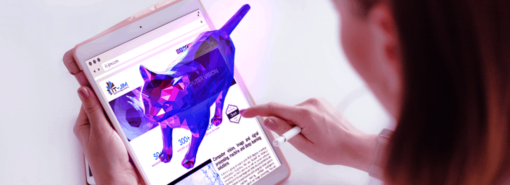
Augmented reality has already proven its positive impact on many businesses. One of the latest trends is so-called WebAR. Indeed, what can be easier than just opening the web page for instant immersive experience?
The goal of this project was to develop and optimize the image detection and tracking algorithm for AR applications. The main challenge was to make it work directly in the mobile web front-end with all computations done on the edge.
To avoid dependence on internet connection and potential lags, we have built an efficient data processing pipeline for web front-end deployment. Firstly, a custom C++ code was developed for content-based image retrieval and tracking. Secondly, we modified and recompiled the C++ code to the WebAssembly binary code using Emscripten SDK to run it directly in the browser. Finally, the algorithm was fine-tuned and optimized within the Emscripten to ensure proper performance on the web.
The image processing engine was just a part of the overall WebAR system. Here is a high-level overview of the created infrastructure:
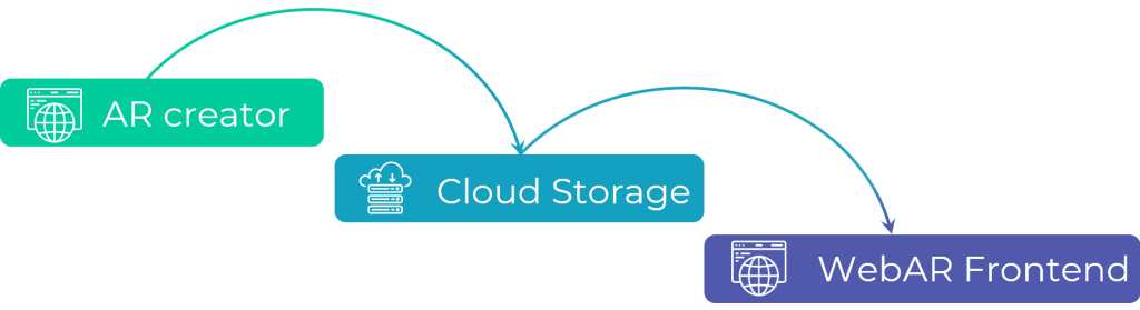
In principle, the architecture of such systems is similar to a common SDKs for mobile AR. The key difference is in the way how it runs in browser. A huge advantage is that you do not need to install any application. Moreover, the WebAR front-end works in both mobile and desktop browsers.
The demo below demonstrates how our WebAR solution works.

If you would like to read more about It-Jim’s WebAR development, please check the blog post and our paper.
Interested in building your own WebAR system or boost your business with cool content in the browser? Let’s discuss! Use the form below to get in touch with us.
A student that is about to graduate from the university and has not yet made up his mind about the career he wants to pursue. A freelancer who has already tried a lot of technologies, knows how he wants to develop himself further and would like to gain experience of working in a company. An experienced IT engineer totally burnt out and aiming to find a new passion. A professional architect (not software one) switching his career entirely.
Do they have anything in common? Yes. All of them have successfully finished It-Jim’s winter internship on computer vision and are now one step closer to achieving their career goals in computer vision and machine learning domains.
Have you ever noticed that the words “winter” and “internship” are made for each other? Or is it just us? The second edition of what we now call “winternship” on computer vision turned out a huge success. We started the campaign in the middle of December 2020, and in three and half weeks we received a truly overwhelming number of applications – 164, a 5x increase compared to the last year! Could we be any happier? Unlike the first edition, this time we had to switch the format to online only due to the ongoing epidemic situation. Yet, we even benefited from it. The geography of applicants this time was quite impressive: Kharkiv, Kyiv, Lviv, Dnipro, Odessa, and many other cities in and outside of Ukraine.
Was it a fun ride selecting the four best candidates out of 164 applications? Most definitely, yes. Especially when there were only 4 spots available. After first filtering the list, we have sent test tasks to 120+ applicants to further narrow down the circle of candidates. Out of 53 participants who tried to solve those tasks we chose 13 persons for interview. Finally, here there were: a student, a freelancer, an IT switcher, and an architect… 4 (w)interns. 4 projects to work on. 4 mentors to guide. 4 weeks to go.

Winternship 2021 Stats
Each of the interns worked on their own project under the guidance of It-Jim’s mentors. We wanted projects that both solved unusual computer vision tasks and were challenging enough for interns, so we opted for the following ones:
Let’s now dive into their realization.
In this project, we wanted to compare two approaches, namely spectrogram analysis and deep learning, for the task of music recognition.
The shazam-like algorithm had the following pipeline:
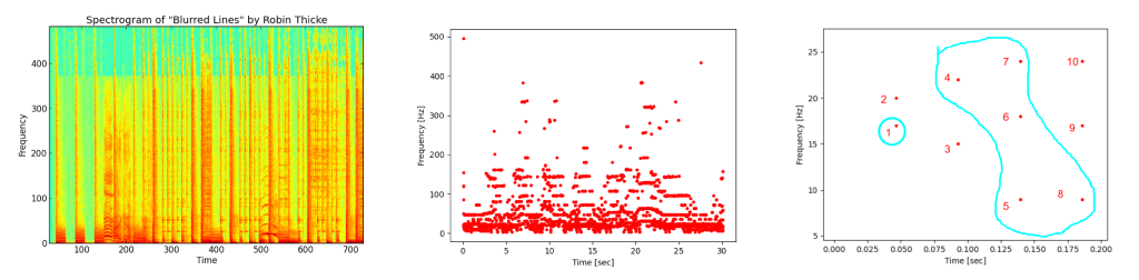
Song spectrogram and its target zone example
The deep learning approach to song similarity estimation had the following steps:
As a result, our intern has demonstrated real-time music recognition for a moderate song dataset. This indicates that audio processing is also about computer vision.
The goal of the project was to develop software that would replace the background behind a person on a video. The core idea was to utilize a monocular depth estimation model to calculate a depth map that can later be used to split the object and background.
An alternative solution was based on the U2-Net model that is usually used for salient object detection. Trained on the Supervisely Person dataset, it managed to give more accurate background replacement compared to the depth estimation approach (see figure below). Also, unlike depth estimation models, it correctly handled cases when a person walked away from a camera view, leaving just an empty background.
After a couple of experiments, our intern provided a real-time demo for background replacement.
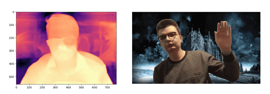
Depth maps predicted by AdaBins trained on NYU (left) and background replacement based on predictions of U2-Net trained on Supervisely Person dataset (right)
The goal of this project was to calculate the heart rate from a video of a person’s face using remote photoplethysmography (rPPG). The latter is based on the blood volume changes in tissue due to the cardiac activity that affects the optical characteristics of reflected light. A proper heart rate measurement is possible only in the case of efficient capturing the changes of red, green, and blue color components. Generally, the rPPG framework consisted of the following steps:
As a result, our intern has provided a real-time demo performing the heart rate estimation from a webcam.

Example of ROI detection (left) and heart rate extraction from the PPG signal (right)
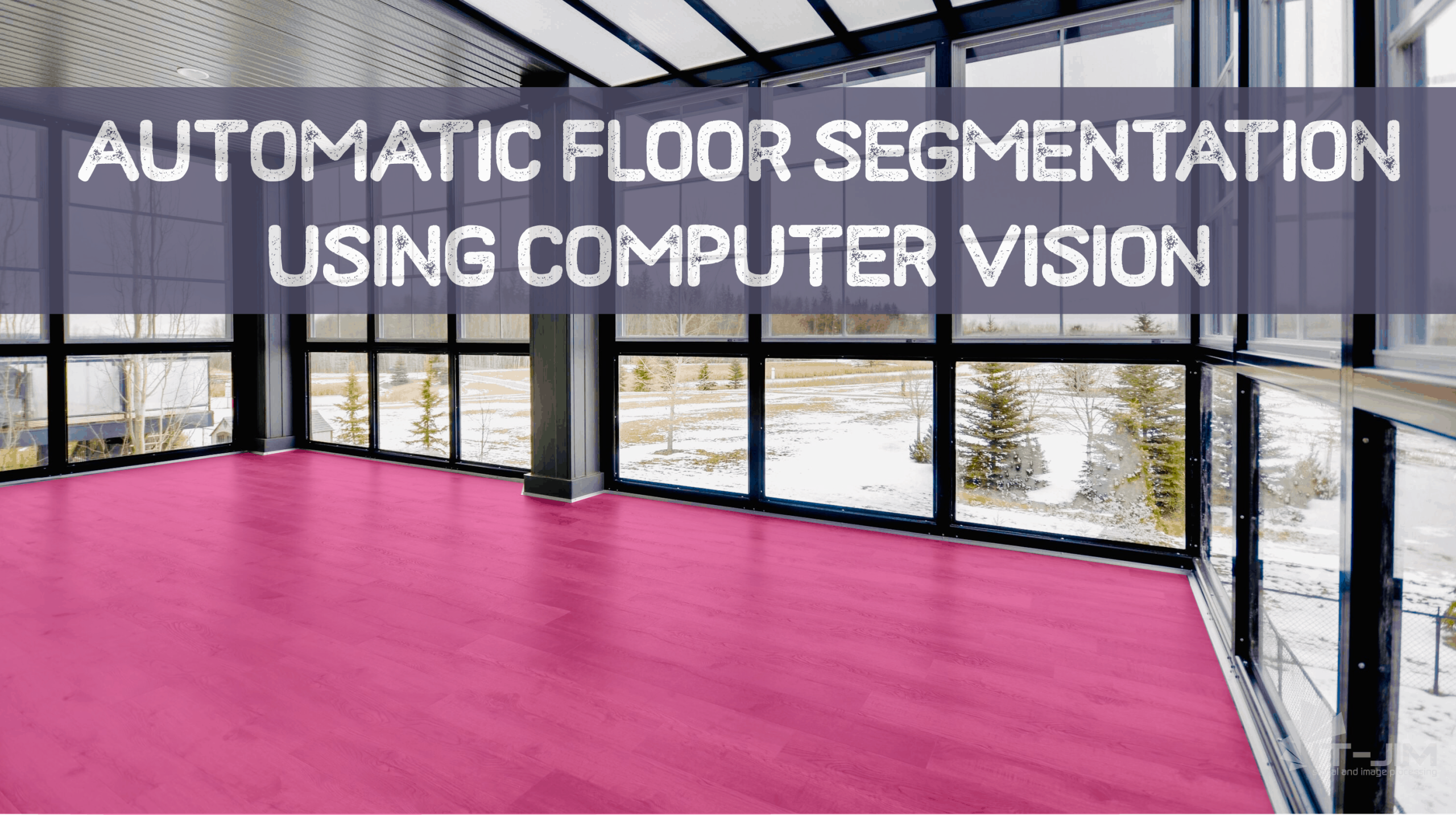
The goal of the final fourth project was to create a pipeline allowing the automatic floor segmentation and replacement in indoor images. We have provided both conventional images from the mobile camera as well as raw data from iPhone’s Pro 12 LiDAR.
Initially, our intern tried to cluster the images using K-means based on pixel coordinates and color components in HSV, RGB and Lab spaces.
As for LiDAR data, we recalculated the raw data into a proper 3D point cloud using the camera intrinsics. Secondly, a RANSAC algorithm was used for the plane fitting.
Finally, a basic fusion scheme was applied to combine the inliers from the RANSAC outputs with merged image clusters.

Depth maps and floor segmentation results
Why do people search for internships? Because it is a perfect way of getting to work on real industrial projects and gaining first-hand experience and mentorship from the experts. It is also a good try-out of the specific field and helps to make one’s mind about the future profession.
Why do we have our internship program? Because we aim at making more people fall in love with computer vision and sharing the knowledge with future generations of engineers.
We organize internships at least once a year. If you missed the last edition, don’t worry: a new type of internship, trainee program, is coming very soon 😉
Automatic floor segmentation can serve many interesting purposes including mixed reality (MR) applications, interior design, entertainment, computation of available space in a room, or indoor robot navigation. In this project, we have been solving a problem of scene understanding and, in particular, determining which pixels of the image belong to the floor.
The problem of floor segmentation is a good example of how the same task can be solved with classical computer vision algorithms or deep learning. As it often happens, the combination of these methods gives the best result.
We start our experiments with superpixels as they are one of the most widely adopted techniques for indoor image segmentation. We use the simple linear iterative clustering (SLIC) that works by clustering pixels based on their color similarity and proximity in the image plane.
Since the straightforward application of superpixels does not provide a perfectly segmented floor, we make a more complex pipeline for image processing. Its steps are illustrated in the figure below and include:
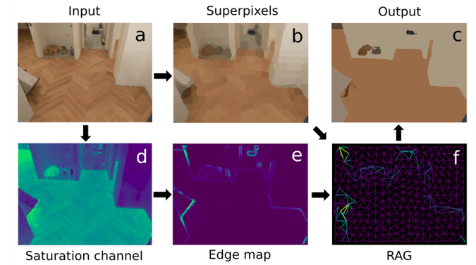
The main steps of the classical pipeline.
The most important step in the classical pipeline is an agglomerative hierarchical merging of the RAG. We analyze edge map intensity between each pair of neighboring superpixels and join those with edge intensity below a certain threshold. We do it iteratively starting from the weakest edges and end up with a few homogeneous regions separated by strong edges. In the figure below you can see the RAG before and after hierarchical merging. All nodes with an edge intensity less than a threshold are merged together. The border of regions is shown in black.
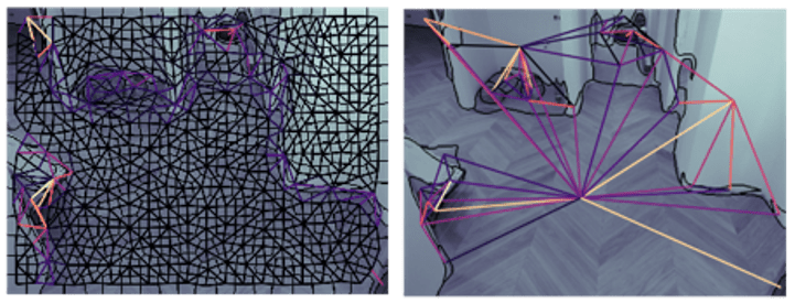
The RAG before (left) and after (right) hierarchical merging.
Since the classical approach is very sensitive to parameter tuning, we have run the classical pipeline several times with different model parameters, resulting in many binary segmentation masks. These masks are joined into a single one by per-pixel majority voting and additional thresholding for balancing precision and recall for a floor class.
The DL solution is based on two CNNs: light-weight RefineNet and FastFCN with a joint pyramid upsampling (JPU) module and modified output layers to predict only 2 classes, a floor and not a floor.
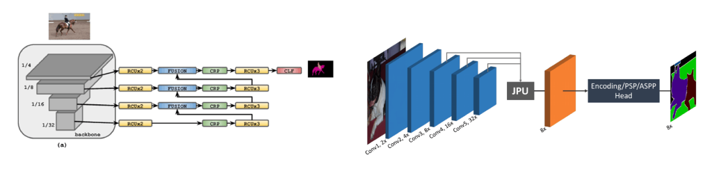
The CNNs architectures used in the paper
For CNN training, we experimented with a few train sets: 1449 images from NYUDv2; 10329 images from the SUN-RGB-D and 8880 images from the SUN-RGB-D with NYUD removed. The target test dataset was a set of 21 hand-labeled images acquired for evaluation purposes.
To additionally refine the quality of segmentation maps, we build a fusion scheme:
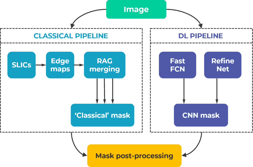
Scheme of classical and DL pipeline fusion.
The binary output mask from the classical branch is combined with the sum of segmentation masks predicted by CNNs, followed by post-processing using texture analysis.
The main purpose of this stage is the final classification of uncertain areas or blobs that result from masks having opposite labels after their summation. Feature analysis resolves these uncertainties and makes a more accurate prediction. In the image below one can see an example with the input image (a), the classical pipeline output (b) the deep learning pipeline output (c) and the resulting mask after post-processing (d).
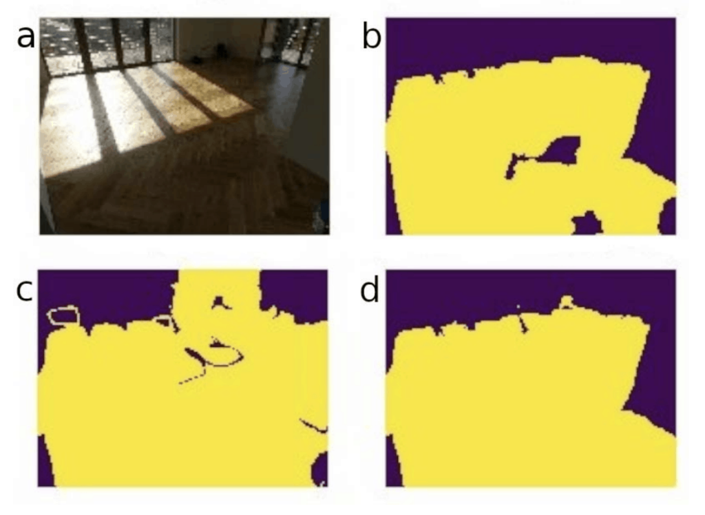
Post-processing based on the texture feature analysis.
For texture features extraction we use a gray-level co-occurrence matrix (GLCM). It determines how often different pairs of pixels appear within a selected region (blob).
To evaluate the results of segmentation we use Intersection over Union (IoU). All intermediate IoU values are shown in the table below.
| Mask obtained with: | IoU |
| Classical branch | 0.5442 |
| RefineNet | 0.7837 |
| FastFCN | 0.7893 |
| Deep learning branch | 0.7939 |
| Classical + deep learning branches | 0.7977 |
| Full pipeline | 0.8013 |
In the following figure, you can find the examples of segmentation masks obtained with the classical pipeline, deep learning pipeline, and as a result of their combination and post-processing.
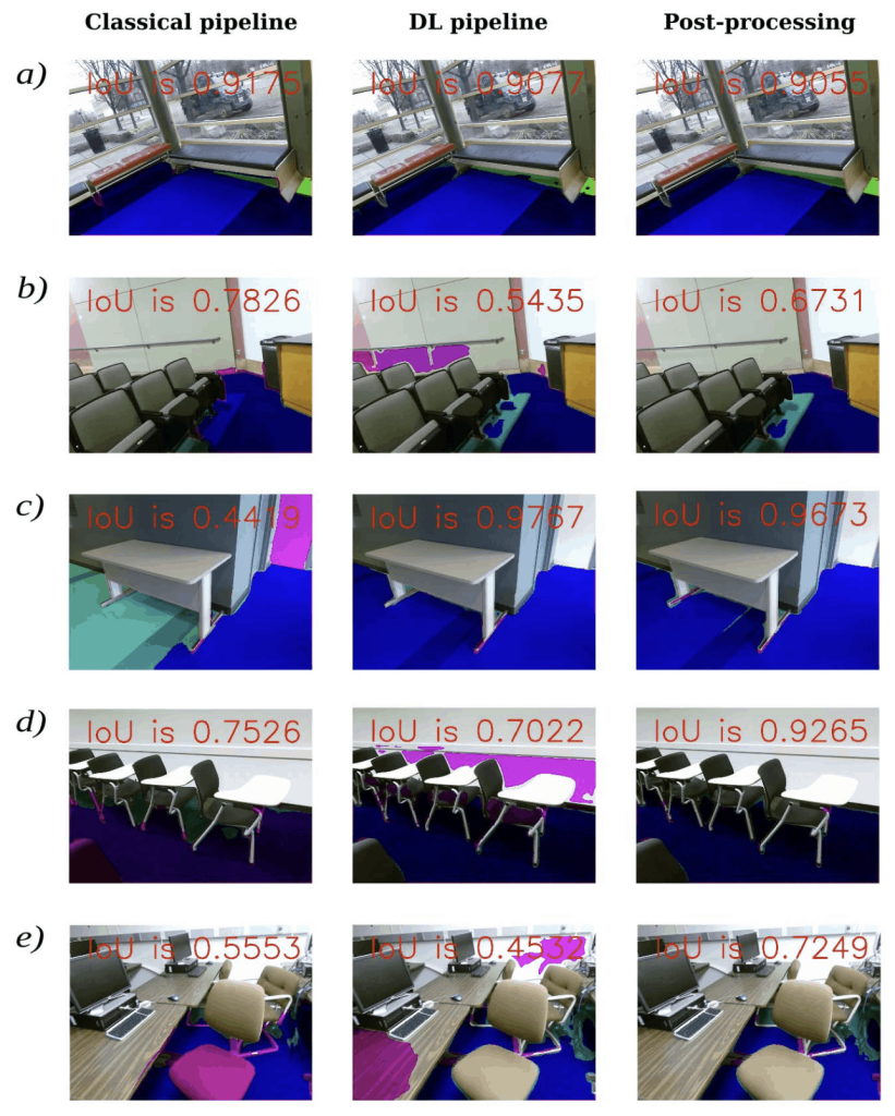
Color legend: dark blue is a true positive, magenta is a false positive, cyan is a false negative.
The deep learning solution handles more challenging cases better than the classical computer vision pipeline. However, for some images, the developed image analysis procedure provides quite competitive results or even outperforms the CNN-based solution. The best result is achieved by merging 3 masks (two from the neural networks and one summed mask from the classical pipeline) and applying the post-processing based on texture feature analysis.
We have examined the problem of automatic floor segmentation. Despite tremendous progress in CNNs, classical CV still does a great job in pre-processing and post-processing stages as well as covers some specific classes where the pre-trained DL model might fail.
If you want to dig into Computer Vision (CV) but have no idea where to start, this beginner guide is for you. Here we recommend some sources which will come in handy for learning and understanding both the computer vision and deep learning basics.
When you search for a position of computer vision engineer, you’re likely to see that companies are looking for a candidate with:
Let’s now go step by step and see how and where to cover each item from the list above:
Do you know what a digital image is? How the color pixels are formed? Have you heard about color spaces, histograms, image filters, and convolution? The video course on digital image processing presented by Prof. Guillermo Sapiro (Duke University) will be a good starting point if you answered ‘No’ to those questions. You can also check the Digital Image Processing tutorial, which is pretty simple but covers a lot. As for the books on the topic, one of the best ones is “Digital Image Processing” by Rafael Gonzalez and Richard Woods. Another book by Ian Young et al. explains the fundamentals of digital image processing and is freely available. As for classical computer vision algorithms, Richard Szeliski’s book “Computer Vision: Algorithms and Applications” is quite comprehensive and has its free draft version available online. Want to dive into the geometry of image formation, projective transformations, or multi-view geometry? Try the course by the University of Pennsylvania on Coursera or “Multiple view geometry” book by Richard Hartley.A hint: Often tutorials on digital image processing use OpenCV examples to gain practical knowledge, so learning this topic might be useful along with exploration of the OpenCV itself (see our recommendations in #4).
When it comes to Maths, you will need linear algebra, calculus, and probability theory. Most likely, you studied them at the university. The good news is that it should be enough. Yet, refreshing the knowledge is always a good idea: an Immersive Math interactive book and video explanations of basic math concepts can help you with this. A nice overview of possible mathematical areas that can be of use for CV is given here. You can always refer to that material if you need a cheat sheet.
If you use C++, keep going, but Python is the most requested programming language in CV/ML/DL . It is easy-to-learn, powerful, and great for CV, ML, and DL tasks. Learn everything from the ground up or level-up your skills with Real Python. There are plenty of free tutorials, structured links to useful resources, and video courses available. An extensive online tutorial from Python developers is another great option to master this skill.
The knowledge of the Numpy library basics is a must-have among your skills. It is used for numerical data preparation and processing. There is a short example-based tutorial to start with. If you prefer video tutorials, check Learn NUMPY in 5 minutes.
Make this open-source computer vision and machine learning software library your best friend. There are plenty of tutorials, you can start with this post to dig in, for example. A comprehensive guide on most of the functions is available as an OpenCV tutorial webpage where you can go on learning digital image processing with examples. You can always check the Learn OpenCV blog for some implemented projects.
Learning ML/DL libraries is useless without theory knowledge. We suggest you start by trying to understand the theory behind the ML algorithms and neural networks first and then implement it with code. Here, it would be a mistake not to mention the classics: Machine Learning course by Andrew Ng on Coursera, The Deep Learning book by Ian Goodfellow. An online book on Neural Networks and Deep Learning by Michael Nielsen may help you, too. Just a kind warning: these are not for kids, maths formulas inside! Stanford University is also offering a couple of extensive lecture series online: Computer Vision (with deep learning) and Convolutional Neural Networks for Visual Recognition. Last, but not least, a recent course from New York University by Yann LeCunn overviews the latest techniques in deep learning and is available both in video and text formats.
Once you have mastered the basics of neural networks and their main parameters to use, it’s time to do some coding. There are two main ways to follow here: using TensorFlow [with Keras inside] from Google or PyTorch from Facebook. Knowing both of them would give you a couple of extra points, of course. Both PyTorch and Tensorflow websites offer quite comprehensive tutorials. To dive into TensorFlow even deeper, try the Hands-On Machine Learning book by Aurélien Géron. An awesome blog PyImageSearch by Adrian Rosebrock can help you a lot. Oldie but goodie AI Shack also counts. Finally, a technical blog of SicaraAI will give you examples of real CV projects.
Now it’s time for practice! If you want to benefit the most, try searching for an internship position or a trainee program. In any case, there are a lot of examples and test datasets on the net, basically on websites from the previous item. You can always enter the competition on Kaggle, collaborate with other engineers to solve real-life problems and get a chance to practice before being employed in the real-world. Try to implement some solutions to have your pet-projects to show on job interviews and jump on board, apply for a position in a CV/ML/DL company!
Well, what else?… Let’s cover some useful tools that can ease your study:
When learning online you can meet the examples or tasks in Jupyter notebooks (wiki) and its online Google colab version. Practically coding there is a bit different from what is usually done in IDE. Knowing the concept of such notebooks could be helpful.
Git now is a standard of a version control system, which is useful not only for professional programmers but helps a lot to download examples from the net, share your projects with others, and demonstrate your experience on job interviews. You should learn the basic terminal commands and understand what’s going on. Modern IDEs usually implement Git commands in their GUI and take care of the routine tasks.
We recommend the PyCharm free community version. It is ok to use simple text editors at first, but you will need more options further. It seems more reasonable to start using IDE and learning its options step by step than switching to IDE when you suddenly realize that your favorite text editor slows down your work.
It’s 2021. AI keeps pushing boundaries and entering new and new areas. The demand for computer vision/deep learning engineers is very likely to keep increasing. Get prepared for this future today 😉
Apple events always amaze the entire world and 2020 was not the exception. Apple presented the first mobile devices equipped with LiDAR: iPad Pro 11 and iPhone 12 Pro (and PRO max version). This active sensor measures physical distances to the objects on a spatial two-dimensional grid. Nowadays it is widespread in the automotive area for object detection and collision avoidance.
How can developers and computer vision engineers use LiDAR in their work? With a lack of technical documentation, there is no other way to answer that question except for making own experiments. In this post, we are going to show you how to create a logger to retrieve data from the iPhone’s LiDAR and an experiment on the accuracy of distance measurements with this scanner. If you want to follow our steps, you’re going to need an iPhone 12 PRO LiDAR, a ruler, a tape measure, and some spare time.

Source: https://www.forbes.com/
First things first. In order to play with the LiDAR data, we need to store it somehow. For this purpose, we created a basic logger application that saves RGB camera frames and depth maps obtained from the scanner.

Screenshot of Logger Application
To use a logger, you need to follow four main steps:
Let’s have a closer look at each of them.
The logger is based on ARSession. It combines data from cameras and motion-sensing hardware to fill an ARFrame object. The latter contains all the necessary information.
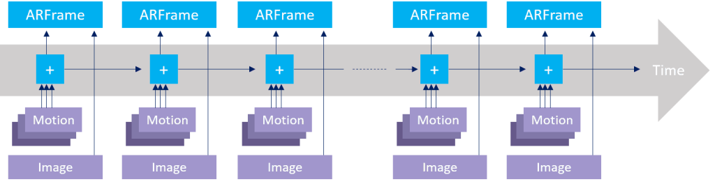
Sensor data storage principle
First of all, we import the ARkit framework into our project. Then we create the ARSession and set up its configuration. This configuration consists of a set of options to enable or disable sensors or tell ARKit how to process given data for a better user experience. As default settings, we choose ARWorldTrackingConfiguration, which tracks changes in translation and rotation of the device (6 Degrees of Freedom).
import UIKit
import ARKit
import Zip

class ViewController: UIViewController, ARSessionDelegate{
    var session: ARSession!

    override func viewDidLoad() {
        super.viewDidLoad()

        session = ARSession()
        session.delegate = self
    }

    override func viewWillAppear(_ animated: Bool) {
        super.viewDidAppear(animated)

        let configuration = setupARConfiguration()
        session.run(configuration)
    }

    func setupARConfiguration() -> ARConfiguration{
        let configuration = ARWorldTrackingConfiguration()

	  // add specific configurations
	  ...
	  return configuration
    	}
}
Since we want to get depth data from LiDAR, we need to check whether our device supports this sensor and enable its flag ‘.sceneDepth’ in ARConfiguration.
func setupARConfiguration() -> ARConfiguration{
    let configuration = ARWorldTrackingConfiguration()

    // add specific configurations
    if ARWorldTrackingConfiguration.supportsFrameSemantics(.sceneDepth) {
        configuration.frameSemantics = .sceneDepth
    }

    return configuration
}
ARSession is ready.
The next step is to capture ARFrame at the specific moment. For this purpose, we added UIButton “SaveFrame” on the display. By clicking on it, you receive the current ARFrame with full information from enabled sensors from ARSession.
@IBAction func onSaveFrameClicked(_ sender: Any) {
    	if let currentFrame = session.currentFrame {
        	let frameImage = currentFrame.capturedImage
        	let depthData = currentFrame.sceneDepth?.depthMap

	      // Process obtained data
            ...
      }
}
This code loads the RGB frame and depth map as ‘CVPixelBuffer’ objects. Additionally, ‘sceneDepth’ contains a confidence map. You might want to take a closer look at it since depth data can be incorrect in the case of surfaces with varying reflectivity.
Let’s now move to prepare the RGB frame and depth map for saving. For that, we convert pixel buffers into ‘UIImages’ in almost the same way. As depth is supported by the limited number of devices, it is an optional type.
if let currentFrame = session.currentFrame {
       ...
      // Process obtained data
      // Prepare RGB image to save
      let imageSize = CGSize(width: CVPixelBufferGetWidth(frameImage),
                            height: CVPixelBufferGetHeight(frameImage))
      let ciImage = CIImage(cvPixelBuffer: frameImage)
      let context = CIContext.init(options: nil)

      guard let cgImageRef = context.createCGImage(ciImage, from: CGRect(x: 0, y: 0, width: imageSize.width, height: imageSize.height)) else { return }
      let uiImage = UIImage(cgImage: cgImageRef)

      // Prepare normalized grayscale image with DepthMap
      if let depth = depthData{
           let depthWidth = CVPixelBufferGetWidth(depth)
           let depthHeight = CVPixelBufferGetHeight(depth)
           let depthSize = CGSize(width: depthWidth, height: depthHeight)

	     ...

           let ciImage = CIImage(cvPixelBuffer: depth)
           let context = CIContext.init(options: nil)
           guard let cgImageRef = context.createCGImage(ciImage, from: CGRect(x: 0, y: 0, width: depthSize.width, height: depthSize.height)) else { return }
           let uiImage = UIImage(cgImage: cgImageRef)
}
While the size of the RGB frame is 1920×1440, the depth map is quite small, only 192×256.
However, even a small resolution of a lidar depth map could be very helpful in object detection or background subtraction tasks.
Depth UIImage is a normalized grayscale image. Distances are encoded in brightness, the closest objects are dark, while the further ones are light.
While for some tasks it is enough to have relative distances, we need to get the real physical values in our case. To get LiDAR distances in meters, we need to read CVPixelBuffer as Float32. In the code below, we fill a 2-dimensional array ‘distancesLine’ with raw depth data.
if let depth = depthData{
    let depthWidth = CVPixelBufferGetWidth(depth)
    let depthHeight = CVPixelBufferGetHeight(depth)
    CVPixelBufferLockBaseAddress(depth, CVPixelBufferLockFlags(rawValue: 0))
    let floatBuffer = unsafeBitCast(CVPixelBufferGetBaseAddress(depth),
				 		to: UnsafeMutablePointer<Float32>.self)

    for y in 0...depthHeight-1{
        var distancesLine = [Float32]()
        for x in 0...depthWidth-1{
            var distanceAtXYPoint = floatBuffer[y * depthWidth + x]
            distancesLine.append(distanceAtXYPoint)
            print("Depth in (\(x),\(y)): \(distanceAtXYPoint)")
        }
        depthArray.append(distancesLine)
    }
		...
Depth data spans from floatBuffer[0] up to [height * width]. In our case, there are 192 rows and 256 columns, 49152 elements in total. Keep in mind that floatBuffer is just a pointer to the memory address with depth information. Like in C++, the pointer does not know anything about the real size of the depth array, so you can easily go out of the limits without any warning.
Finally, we need to save our results to the device folder to have an opportunity to analyze them. The following auxiliary code creates a folder, gets its path, and clears the folder in case it was built before.
func getTempFolder() throws -> URL {
    let path = try FileManager.default.url(for: .documentDirectory, in: .userDomainMask, appropriateFor: nil, create: true
).appendingPathComponent("tmp", isDirectory: true)

    if (!FileManager.default.fileExists(atPath: path.path)) {
       do {
           try FileManager.default.createDirectory(atPath: path.path, withIntermediateDirectories: true, attributes: nil)
       } catch {
               print(error.localizedDescription);
       }
    }
    return path
}


func clearTempFolder() {
    let fileManager = FileManager.default
    let tempFolderPath = try! getTempFolder().path
    do {
        let filePaths = try fileManager.contentsOfDirectory(atPath: tempFolderPath)
        for filePath in filePaths {
            try fileManager.removeItem(atPath: tempFolderPath +
                                               filePath)
        }
    } catch {
            print("Could not clear temp folder: \(error)")
    }
}
The folder should be created when setting up our ARSession.
override func viewDidLoad() {
    	super.viewDidLoad()

    	clearTempFolder()

    	session = ARSession()
}
Now, we can save images and depth array as a .txt file.
// Save image (the same for depth)
let imagePath = try! getTempFolder().appendingPathComponent("\(frames.count).jpg")
try! uiImage.jpegData(compressionQuality: 0.9)?.write(to: imagePath)


// Save depth map as txt with float numbers
var depthTxtPath=try! getTempFolder().appendingPathComponent("\(frames.count)_depth.txt")
let depthString:String = getStringFrom2DimArray(array: depthArray, height: depthHeight, width: depthWidth)
try! depthString.write(to: pathTxt, atomically: false, encoding: .utf8)


// Auxiliary function to make String from depth map array
func getStringFrom2DimArray(array: [[Float32]], height: Int, width: Int)->String{
    var arrayStr: String = ""
    for y in 1...height-1{
   	 var lineStr = ""
   	 for x in 1...width-1{
   		 lineStr += String(array[y][x])
   		 if x != width-1{
   			 lineStr += ","
   		 }
   	 }
   	 lineStr += "\n"
   	 arrayStr += lineStr
    }
    return arrayStr
}
Now we are ready to compare the measured depth by LiDAR with real physical distances to objects. ARKit documentation suggests avoiding highly reflective or light-absorbing surfaces. The company’s poster meets these requirements perfectly, so we used it as a target. We fixed a smartphone with a tripod and centered the object on the screen.
 |
 |
Scene configuration
As long as we were dealing with a flat and distributed object, it was enough to take the data just from the central pixel of the depth map. We recorded the LiDAR data for distances from 20 cm up to 5.5 m. We used a 5 cm measurement step for distances up to 1 m and a 50 cm step for the larger ones. The distance was captured by LiDAR a few times to evaluate the repeatability of the results. Here is what we obtained.
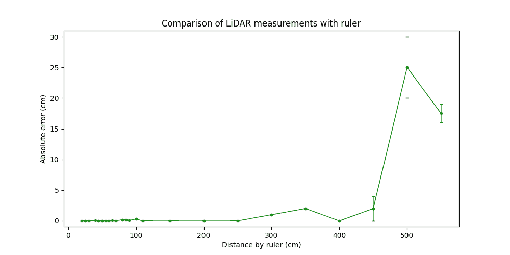
Experimental results
One can see that LiDAR provides reasonable accuracy for distances of up to 4 meters which is sufficient for portrait mode and short-range AR. The higher distances provided different results for every button click (see error bars in the figure above). This indicates the limits for the iPhone’s LiDAR operation range.
Definitely, the iPhone Lidar sensor is interesting to play with. We hope that provided code snippets and findings will be useful for those who are willing to examine the new LiDAR sensors. Our iPhone experiments are definitely to be continued. Stay tuned!