Get Ready to Dive into AI with Our New R&D Lab

Join Our R&D Lab and Take Your AI Skills to the Next Level!

It-Jim is excited to announce the launch of our brand-new R&D lab, where you can work on real projects, collaborate with experienced engineers, and dive into cutting-edge AI research.

Our R&D lab focuses on multimodal AI applications, 2D/3D computer vision, generative AI, and AI-powered mobile development. By joining our lab, you’ll work with the latest AI technologies and techniques while sharpening your Python and C++ skills. You’ll collaborate with experienced engineers, project managers, and tech leads to create groundbreaking AI solutions.

This position is perfect for anyone with 1+ years of experience in IT or previous involvement in AI projects who wants to excel and take their skills to the next level. We’re looking for passionate and curious individuals. The ideal candidates should have a strong foundation in Python, basic knowledge of C++, and be familiar with deep learning frameworks. Previous work experience in an IT company or involvement in AI projects is highly valued.

The program is a full-time engagement, and we offer a negotiable salary. You’ll get the chance to work on projects that will shape the future of AI and be part of a vibrant community of like-minded people.

“We believe that investing in talent is key to advancing the field of AI and developing innovative solutions that will improve people’s lives,” said It-Jim’s CEO, Ievgen Gorovyi. “That’s why we’re launching our R&D lab and inviting all AI enthusiasts to join us on this exciting journey!”

Don’t miss this opportunity to take your AI skills to the next level with a full-time engagement. Apply now and learn more about the lab ⬇️

Join our AI R&D lab today:

https://www.it-jim.com/careers/ai-rd-lab/

AI-Powered Mobile Development

The iPhone isn’t just a device for consumers – it’s also a powerful computational unit with a wide range of sensors and hardware that’s ideal for running machine learning algorithms. By leveraging this capability, businesses can enjoy low-latency performance, local inference, and significant cost savings by avoiding cloud infrastructure fees. At It-Jim, our team of mobile AI developers is here to help you harness the power of the iPhone for your business needs.

iOS as a Platform for Edge Computing

The iPhone’s hardware, Apple Neural Engine, coupled with our expert utilization of iOS frameworks, allows us to perform instant data analysis and deliver meaningful results in a wide range of industries – from sports and healthcare to entertainment, retail, surveillance, and even automotive.

Our goal is to transform your mobile device into a powerful tool that delivers real value, without the need for costly hardware upgrades. With countless fascinating use cases, we’re excited to help you explore the limitless potential of iOS-powered edge computing.

iPhone as a 3D Scanner

Did you know that your iPhone can be used as a high-precision 3D scanner? By utilizing its camera and LiDAR sensor, we can create accurate 3D maps of your surroundings and reconstruct objects with incredible detail. And the best part? This 3D reconstruction process can be done right on your device, opening up a world of possibilities such as:

  • Texture reconstruction and recognition
  • 3D object detection and tracking
  • Floor plan and room layout extraction
  • 3D measurement of object shapes and dimensions
  • Object visual inspection

We make use of all available iOS frameworks for real-world perception, 2D/3D data processing, machine learning, and AR.

3D and AR iOS frameworks we typically use: ARKit, RealityKit, SceneKit, Roomplan, MetalKit, GL Kit, Model I/O

CV and DL iOS frameworks: CoreML, Vision, CoreImage, CoreVideo, CoreMotion, CreateML, AVFoundation

By combining the powerful iOS frameworks with custom computer vision, deep learning, and sensor fusion algorithms, we can transform your iPhone into a powerful 3D scanner. This technology has incredible potential across a wide range of industries, from design and augmented reality (AR) games to construction and insurance.

At It-Jim, we’re committed to helping you harness the full potential of 3D data processing to take your business to the next level. We’ll help you leverage the latest in mobile technology and custom algorithms to unlock new insights and opportunities that you may not have even considered before.

iPhone as a Smart Microphone

With the explosion of audio, speech, and sound processing technology, your business can benefit from our R&D team’s expertise in this area. We are experts in a range of directions, including 

  • automatic speech recognition (ASR) or speech-to-text (STT), 
  • text synthesis or text-to-speech (TTS), 
  • emotion recognition, voice biometrics, and liveness detection, 
  • sound classification, speech enhancement, and noise suppression.

Our exceptional team of PhDs and software engineers can provide you with the best solution, no matter where you want to utilize the power of audio processing. We work with businesses across a range of industries, including healthcare and wellness, media, social networking and podcasting, gaming, marketing, and more.

At It-Jim, we develop custom solutions that do the job directly on the device to achieve zero latency, maximum security, and cost-effectiveness. We optimize the accuracy and performance tradeoff, leveraging the available ML models and CoreML framework while developing custom algorithms in C++ when needed.

iPhone as a Navigation Sensor

The iPhone’s sensors (cameras, LiDAR, accelerometer and gyroscope) offer a range of possibilities for location retrieval and navigation, making it a versatile tool for GPS-denied environments such as multi-level parking, business centers and exhibitions. What’s more, you can add an AR layer and transform your iPhone into a portal to the digital world that erases the borders between real and virtual environments.

Our team at It-Jim can leverage the following solutions for visual localization and tracking, including:

  • Visual SLAM and VPS
  • ARKit and custom user localization
  • Incorporation of fiducial objects, such as QR codes, images, or 3D objects, as anchors
  • Bluetooth Low Energy (BLE) and Inertial Measurement Unit (IMU) for indoor navigation
  • Multi-sensor setup for distributed areas (SLAM+BLE)

All above is possible with a core functionality implemented on your iPhone. This allows for efficient and cost-effective business applications without the need for additional hardware.

iOS Development for Pattern Recognition and Image Processing

Get ready to be amazed by what your iPhone camera and our AI expertise can do! With the help of the It-Jim team, your device can be transformed into a powerful tool for pattern recognition and image processing. Here are just a few examples of what your iPhone can be transformed into:

  • An efficient barcode scanner that can read 1D barcodes, QR codes, and perform custom pattern recognition.
  • An optical character recognition (OCR) tool that can extract text from images with high accuracy.
  • An instrument for real-time visual search that can recognize and categorize objects in real-time.
  • A device for quantitative estimation of biomarkers, providing lab-grade accuracy in the comfort of your own home.
  • A precise optical sensor working with the pro-RAW image format, providing unparalleled image quality and flexibility.

Our AI team has the expertise to get the maximum benefit from the advanced sensors in iOS devices, eliminating the need for external hardware in many cases. Let us help you unlock the full potential of your iPhone for pattern recognition and image processing.

iPhone for Video Processing and Analytics

Video processing and analytics on an iPhone can offer a multitude of benefits as well. It-Jim team can help you achieve the following use cases:

  • Recognizing emotions in videos
  • Tracking scenes and objects for augmented reality applications
  • Applying video effects such as inpainting and watermark erasing
  • Implementing AI-driven facial analysis for AR masks, toonification, emotion recognition and analytics, vitals estimation, face swap, face detection and recognition
  • Creating virtual try-on applications for hair, glasses, and clothing

We have the expertise to capture, process, encode/decode, compress, and analyze video streams with maximum efficiency. Our team can also distribute computations between the edge and cloud to optimize performance. With our expertise, you can rest assured that your business will benefit from cutting-edge video processing and analytics capabilities, all powered by your iPhone.

Ready to take your business to the next level with AI-powered iOS app development?

Text Prompt Engineering for Image Generation

The development of modern neural networks has brought about a revolution in the field of image generation. One such example is the text-to-image neural network, DALL-E 2, which can generate beautiful art when supplied with good text descriptions (typically referenced as “prompts”).

Project Description

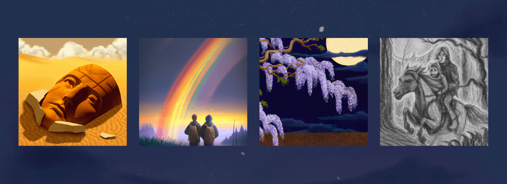
The quality of images generated by DALL-E 2 heavily depends on the proper structure of inputs. But what if one has a poem and wants to generate a matching art for it without learning all intricacies of writing good prompts? That is exactly what our client was looking for. Our team recognized this challenge and leveraged our experience with GPT-3, a powerful large language model, to create an automatic prompt generator for DALL-E 2. The combined pipeline of GPT-3 and DALL-E 2 allows a user to get wonderful images given only a poem itself, just as if they have a professional prompt engineer to help them.

Solution

One of the key challenges we faced in developing this solution was the lack of a dataset of poem-prompt pairs. To overcome this, we had to use either a zero- or few-shot learning approach. We have tested multiple prompts for GPT-3 and accompanied the best one with examples of good DALL-E 2 prompts. The example prompts were designed to resemble those typically used for literature illustrations and were randomized each time to reduce the likelihood of repetitive results.

Here are some examples of how our solution works:

The solution we developed was delivered to our client as a web application, with deployment on AWS. This powerful tool allows anyone to generate stunning artwork based on a poem without the need for any prior expertise in prompt engineering.


How Text-to-Speech Models Work: Theory and Practice

Text-to-speech (TTS) has been a popular topic for some time, and its development shows no signs of slowing down. There are a plethora of deep learning models, software programs, and companies offering this service. It’s no surprise, given the broad range of applications, from voice assistants and answering machines to creating audio versions of articles, books, and even automatic voiceovers for videos. Consequently, developers strive to improve the quality of these systems by creating more natural-sounding voices that are indistinguishable from human speech.

This blog aims to describe and compare the best open-source text-to-speech models and Python libraries that are easy to use. If you’re curious about how these models work, we’ll briefly explain the theory behind them and their structure. If you’re here to quickly learn how to use them in Python, feel free to skip ahead to the corresponding paragraph about the VITS model. This model provides fast, real-time text-to-speech synthesis with over 100 pre-trained voices. Alternatively, if you’re interested in good-quality voice cloning, the paragraph about Tortoise TTS may pique your interest. Please note, however, that this is a slow model.


Text-to-speech explained

To begin with, let’s clarify what a text-to-speech model is. TTS, or speech synthesis, is a system that takes text as input and generates an audio signal from it. The primary goal of modern TTS is to make a synthesized speech from text sound not only comprehensible but also natural. However, achieving a high level of naturalness is often subjective and evaluated using metrics such as the Mean Opinion Score (MOS). MOS is a subjective rating obtained from human listeners who evaluate synthetic speech samples generated by the TTS system. Listeners rate speech samples on a scale of 1 to 5, where 1 represents poor quality, and 5 represents excellent quality. The scores from multiple listeners are then averaged to determine the overall MOS for the TTS system. It’s worth noting that MOS is usually calculated when a model is trained on the LJspeech, the most popular open and free-to-use dataset. However, even original samples from this dataset do not receive a five-score evaluation.

Let’s take a deep dive into the theory of TTS models. Typically, modern deep learning TTS models consist of three essential components:

  • a text analysis module (also known as the frontend),
  • an acoustic model, and
  • a vocoder.

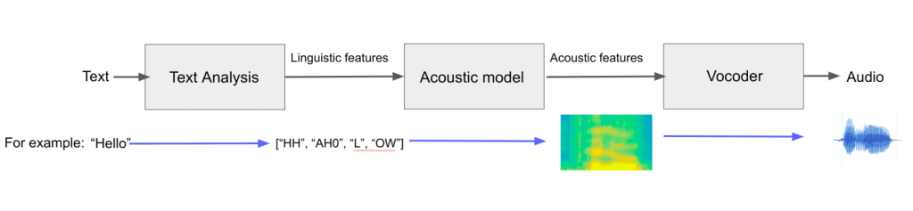
The text analysis module converts a text sequence into linguistic features. The acoustic model generates acoustic features from those linguistic features. Finally, the vocoder synthesizes a waveform from those acoustic features. Of course, there are many different types of each of these components, and if you want to dive deeper into the various acoustic and linguistic features and their representations, I highly recommend checking out this survey about TTS models. To give you a better idea of how the system works, look at the basic visualization of such a system in Fig. 1. Here, the text analysis module has phonemes as output, and the acoustic model produces a mel-spectrogram.

Fig 1. Basic components of a TTS model.

While the abstract diagram of the TTS model may appear straightforward, each of its components has a much more intricate structure. The field of TTS boasts numerous text-to-speech models and vocoders, including Tacotron2, FastSpeech2, Glow-TTS, VITS, HiFi-GAN, MelGAN, and WaveGlow, among others. It is worth noting that if these models share the same acoustic features, such as the mel-spectrogram, it is possible to combine the acoustic model from one TTS with another vocoder in some cases. Figure 2 illustrates the data flows of various TTS models available as of July 2021.


Fig. 2 The data flow from text to waveform and different models from the survey on TTS solutions.

One example of an end-to-end TTS model that leverages this approach is VITS, which combines the GlowTTS encoder and HiFi-GAN vocoder. While the underlying theory of TTS still applies, VITS has demonstrated superior performance compared to other models. In fact, its MOS output on the VCTK multi-voice dataset achieves a ground truth level. If you’re interested in trying out this fast TTS model, read on for a practical guide on how to use it.


Voice Cloning

The field of voice cloning is a challenging subfield of TTS. Its goal is to generate speech that closely matches an audio reference voice. If you have a significant amount of audio data of the voice you want to clone, you can train any TTS model on it. However, a different approach is needed if you have only a few samples. Fortunately, there is one – Tortoise TTS, a model specifically designed for high-quality voice cloning.

Tortoise TTS consists of five separately trained neural networks that are pipelined together to produce the final output. Its components draw inspiration from image generation models such as DALL-E and denoising diffusion probabilistic models. The production of the final waveform has the following steps:

  • Text input and reference clips are fed to the autoregressive decoder that outputs latents and corresponding token codes representing highly-compressed audio data. This step is repeated several times to produce multiple “candidate” latents.
  • The CLVP (Contrastive Language-Voice Pretraining) and CVVP (contrastive voice-voice pretraining) models select the best candidate. The CLVP model produces a similarity score between the input text and each candidate code sequence, while the CVVP model produces a similarity score between the reference clips and each candidate. These two similarity scores are combined with a weighting provided by the user, and the candidate with the highest total similarity proceeds to the next step.
  • The diffusion decoder then consumes the autoregressive latents and reference clips to produce a mel-spectrogram representing the speech output.
  • Finally, a UnivNet vocoder is used to transform the mel-spectrogram into actual waveform data.

TortoiseTTS was called this way for a good reason – the model is very slow, and running it on a GPU is highly recommended. However, its ability to produce high-quality voice cloning results with only a few reference audio samples makes it a valuable tool for many applications.


Practical Guide: VITS

In this practical guide, we will show you how to use the VITS model to synthesize speech with the CoquiTTS library in Python. This library contains:

  • acoustic models: Tacotron, Tacotron2, Glow-TTS, Speedy-Speech, Align-TTS, FastPitch, FastSpeech, SC-GlowTTS, Capacitron, OverFlow,
  • vocoders: MelGAN, MultiBandMelGAN, ParallelWaveGAN, GAN-TTS discriminators, WaveRNN, WaveGrad, HiFiGAN, UnivNet,
  • and two end-to-end TTS models: VITS, YourTTS (based on VITS).

From our experiments, VITS produces the most natural results and works with low RTF (real-time factor), even on the CPU.

If you are not planning to train this model, to get started, install the CoquiTTS library using pip:

pip install TTS

Once you have installed the library, synthesizing speech is straightforward. Here is an example code snippet that generates speech from a text input using the VITS model:

 
from TTS.api import TTS 

text = 'Hello, dear readers of the blog about TTS models!' 
model_name = 'tts_models/en/vctk/vits' 
speaker_id = 77 

tts = TTS(model_name) 
tts.tts_to_file(text=text, speaker=tts.speakers[speaker_id], file_path='output.wav') 
# tts.tts(text=text, speaker=tts.speakers[speaker_id]) 


In the code above, we first define the input text, model name, and speaker ID. We then create a TTS object using the VITS model and use the tts_to_file method to synthesize speech and save it to a file. If you want to use the output as a signal instead of saving it to a file, you can use the tts method instead of tts_to_file. The sampling rate of the result = 22050 Hz.

Note that the first time you run this code, the model will be downloaded to your machine, and in the future, it will be used automatically. You can try more than 100 voices from the VCTK dataset by choosing the corresponding speaker_id. There are both female and male voices with different accents.

CoquiTTS repository: link

Listen to the result examples:

Male voice:


Female voice:


Practical Guide: Tortoise TTS

You can use Tortoise TTS in the official Google Colab. However, this practical guide will help if you want to run it locally. We will start by preparing the environment and the reference audio, then we will split the reference audio into small clips and finally, we will use Tortoise TTS to clone the voice. Let’s get started!

First, you need reference audio to clone the voice – so make sure you prepare reference audio or video where only one person is speaking. It can be 10 seconds or longer, we will split it in the code.

Now, let’s create a separate conda environment and activate it. Install the repository:

git clone https://github.com/neonbjb/tortoise-tts.git
cd tortoise-tts
python -m pip install -r ./requirements.txt
python setup.py install

In addition, install pydub, which will help us to create an audio clips from video or audio file.

pip install pydub

Let’s import functions and libraries that we will use:

import torchaudio
import os
import math

from tortoise.api import TextToSpeech
from tortoise.utils.audio import load_voice
from pydub import AudioSegment


It is recommended to split reference audio into small 6-10 second audio clips. Here is a simple function that will split audio if it is longer than 12 seconds into small clips and save them to the voices folder.

def prepare_voice(voice_name, path_to_original_voice):
    custom_voice_folder = f"tortoise/voices/{voice_name}"
    os.makedirs(custom_voice_folder)

    full_audio = AudioSegment.from_file(path_to_original_voice)
    duration = len(full_audio) / 1000

    if duration < 12:
        full_audio.export(os.path.join(custom_voice_folder, f'{0}.wav'), format='wav')
        return

    amount_of_parts = math.floor(duration / 6)
    part_duration = len(full_audio) / amount_of_parts

    for i in range(amount_of_parts):
        part = full_audio[i * part_duration:(i + 1) * part_duration]
        i += 1
        part.export(os.path.join(custom_voice_folder, f'{i}.wav'), format='wav')


Run this function with your parameters, where voice_name is the name of a new voice, path_to_original_voice is the path to the video or audio with the voice you want to clone.

Finally, we can create the speech from text with voice cloning (don’t forget to change the voice_name):

voice_name = ‘custom’
text = ‘Hello, dear readers of the blog about TTS models!’
output_path = ‘output.wav’

tts = TextToSpeech()
preset = "high_quality"

voice_samples, conditioning_latents = load_voice(voice_name)
audio_signal = tts.tts_with_preset(text, voice_samples=voice_samples, 
                                   conditioning_latents=conditioning_latents, 
                                   preset=preset)

torchaudio.save(output_path, audio_signal.squeeze(0).cpu(), 24000)


And that’s it! With these simple steps, you can use TortoiseTTS to clone a voice from reference audio.

Official repository: link

Listen to the result examples (Both examples took approximately 30 min each to run on the local GPU):

Voice of Amy Winehouse, cloned from the 30s of this interview.


Voice of Jordan Peterson, cloned from the 30s cut from this video.


Conclusions

The conclusions of this article highlight the accessibility and ease of use of modern TTS systems. Whether you’re a developer looking to integrate TTS into your projects or a content creator seeking to produce audio content, there are a variety of TTS tools available to suit your needs. From the VITS model in the CoquiTTS library to the slower but higher-quality TortoiseTTS, TTS technology has come a long way and continues to evolve, promising exciting advancements in the future.


Top 9 iOS Applications for 3D Reconstruction

People are excited about extended reality. They dream of having a Metaverse where they would spend their time and earn money. And one of the key aspects of the Metaverse is the virtual world itself. It may be designed by artists, created via procedural 3D modeling, or taken from the real world via scanning. The broader availability of consumer 3D scanning makes it one of the most promising ways for the massive generation of the Metaverse.

How a 3D model is created

3D mapping creates a 3D model of physical objects. It can be achieved in various ways, for example, by using a professional lidar scanner. Or you can do that with the lidar of the new iPhone. Alternatively, one may use the SfM (Structure from Motion) approach, where a stack of photos of the same space or object is fed to an algorithm that solves the optimization problem where camera positions and 3D point locations are the optimized variables. That process outputs a point cloud that transforms into a 3D model after densification and meshing.

The models differ in their precision, level of detail, and presence of textures. Those depend on the quality and quantity of input images, the algorithms involved, and the computational effort spent. Recently, a number of apps have been introduced offering 3D scanning of fair quality for consumer smartphones. It is much more convenient than using professional equipment, which is typically a way to generate a 3D scan.


The quality gaps between apps reflect a structural constraint: all automated reconstruction methods produce dense, unoptimized geometry that needs cleanup before it is usable in a game engine, product renderer, or manufacturing workflow. Our article AI 3D Generation: From Prototype to Production covers that post-processing pipeline for AI-generated 3D geometry. The same logic applies to everything compared here.

What were we evaluating in the reviews?

As a computer vision company, It-Jim is fascinated by the new possibilities which appear along with the lidars for consumer devices. We’ve tested several 3D lidar-based scanning applications for iPhones and want to share the results. Our list of 3D apps to examine included Scandy Pro 3D scanner, Qlone 3D scanner, Cubicasa, Matterport Capture, Magicplan, 3D Scanner App, Polycam, Mapstar, and Scaniverse. Our primary interest was the quality and speed of reconstruction. We’ve also checked the usability of the apps as well as additional features like large object and small object scanning modes, export, ease of registration, and cost. The table below summarizes our high-level marks (10-point scale, where applicable).

Features UX Large object mode Small object mode Export Registration Price Social network in the app
Scandy Pro 3D scanner 3 8 + 5 $ 150 or signup
Qlone 3D scanner 2 3 + + free or $ 15
Cubicasa 5 5 + $ complicated $ 10 per model
Matterport Capture 4 7 + + free
Mapstar 5 3 + complicated free +
Magicplan 9 9 +/- + free or $ 10
3D Scanner App 8 8 + + 10++ free
Scaniverse 10 10 + + 7 free
Polycam 10+ 10+ + + 10++ + free +

The technology is not yet perfect, so each app has its drawbacks and limitations. Let’s cover them in detail.

Scandy Pro 3D scanner

7-day free trial. Features: 3/10. UI/UX: 8/10

Scandy Pro 3D scanner is an application whose main function is the 3D reconstruction of spaces. And, broadly speaking, it does the job. How well and is it convenient enough? The question remains open.

It’s important to note that we were only able to run the app with a selfie camera and TrueDepth sensor (that is, without the main camera and lidar). At the time of writing this review, some changes have been made to the app.

What’s not right?

The nuisance that immediately catches your attention is the vibration you get for “incorrect scanning.” However, the app doesn’t provide any explanation on how to do the scan right. In addition, the app behaves strangely before you press the “scan” button. Also worth noting is the loss of camera position tracking even in relatively simple cases

About models 

Even if you manage to scan a surface, the app is likely to lose about 70% of it. In the preview, the grid shows more than in the final version. The resulting model can be edited, saved, and sent – no other options for working with it are available. 

An odd feature 

As for the face scanning, it was, again, not without “surprises.” For a successful scan, the user must turn his head smoothly and slowly in front of the camera. Partial visual control of the process greatly complicates the task. 

Any pros to the app? 

Yes, there are some, too. We can note a fairly fast display of the scanned surface and the ability to export to 5 file formats. But of course, this doesn’t positively affect the user experience in the application.

Qlone 3D scanner

Free/$15. Features: 2/10. UI/UX: 3/10.

In general, the app has some apparent limitations and a rather poor scanning, although it has some good sides to it, too. 

To begin with, mappable objects are small and limited. Which is to say, this scanner is not suitable, for example, for the reconstruction of spaces. 

The user must print the background mat. Moreover, the size of the object for 3D must be comparable to the size of the printout. At least the user can print the background from the application directly. 

About the scanning process

As for the scanning itself, it is quite disappointing. The free version works with a helping marker. The user should print this marker and place the object on that. The user must cover all sectors augmented around the marker. The scanning process requires patience and effort. 

The only thing we can highlight as a plus is fair scanning interactivity.

Cubicasa

Free/$15. Features: 5/10. UI/UX: 5/10.

In this case, we had to place an order (starting at $9.99) to get the scan results and thus be able to write an app review in full. We didn’t do that since there are plenty of free options. 

Getting Started challenges

To get started with the app, you need to register. The registration process is lengthy as it requires a lot of information: about the company, the type of user, etc. When using the application, the unreasonably large buttons in the menu strike the eye, which is not necessarily a downside but rather a UI flaw. 

App functionality:

The developers claim that there’s a 3D room reconstruction among the app’s functions. Scanning is available, and an augmented mesh is also shown. Each scan requires typing in some information. That is not user-friendly. The album mode for capturing is not comfortable. 

In-app Tutorials

The scanning tutorial is supposed to simplify the process, but to find the answer, you must go through multiple pages. Still, the warnings and tips for scanning are reasonably well-designed and helpful. 

To sum up, the app has some pretty nice features, but it can hardly be called entirely user-friendly.


Matterport Capture

Free. Features: 4/10. UI/UX: 7/10.

One example of a fair-quality and easy-to-use application, which, of course, is not without its limitations. 

The main features

The menu and functionality are made simple and accessible to a wide range of users. It is important to note a good tutorial of the application.

When scanning, you have to point the camera at some AR markers added to the frame. This could be a good helping feature. The app can generate a 360-degree panorama. In addition, a room plan with a view from the top is available. 

Some difficulties in the use

Scanning is limited to panorama mode – the user has to rotate the phone while holding the camera in the same place (which is not that easy). 

We could not extract any 3D objects while using the app.

Mapstar

Features: 5/10. UI/UX: 3/10

The dream of the authors of the Mapstar app is to create a meta-universe using scanning, geolocation, and NFTs. The app contains a specific “social” network with other users’ creations. Among the main features, 3D reconstruction tools are available both with and without lidar. In addition, there are some additional features whose usability might be questionable. 

App Functions and difficulties in using them 

The application cannot be used without registration. But the actual problem is that the registration process itself has a lot of bugs, which creates difficulties right from the start.

The lidar scan is hard to call high-quality. A feature which makes Mapstar app different from the others in a good way is that it is able to make scans without lidar which works quite well considering the limitations of non-lidar data. One of the features of the models is the ability to add 3D effects and links from YouTube. 

Some objects are not scanned, such as a single-color ceiling. In addition, the preview picture often looks nice, but as a result, we get a model with many flaws and discrepancies.

Unfortunate visual solutions

As for the visual aspect of the application, there are things that could be improved here as well. Visually, it looks raw. The design, UI, and UX have many shortcomings that make the app difficult to use and not particularly attractive. It’s also inconvenient to view added photos and videos because of the unfortunate design solution. 

The preview grid creates visual clutter during scanning, which does not add to usability. In addition, the mesh takes quite a long time to initialize. 

There are other oddities of the app as well. For example, the main screen displays a reconstruction made by some random user. It’s not quite clear why this solution was implemented.

Magicplan

Free/$9.99. Features: 9/10. UI/UX: 9/10.

The main purpose of the application is to create floor plans, which are drawn using a user interface. The application can even be used for large-scale projects, such as a 50-floor building. 

A first look at the app

It’s worth noting that it was designed to create 3D sketches, not 3D reconstructions. The functionality of the app is great for 3D apartment design. Users can also create a 3D sketch without scanning.  

What really stands out when you first look at the app, is the well-made user interface. It is visually satisfying, but it also has useful tips and hints. Thanks to the capabilities of the application, you will be able to predict quite accurately what the renovation will look like — paint type and amount, installing of doors and sinks, large choice of furniture with variation. The app demonstrates an excellent implementation of the possibility of creating a room model by points.

What’s in the app?

Scanning is limited to highlighting flat walls and corners and thus measuring room’s shape. The corners of the room are detected automatically. The resulting models can be edited by changing the color, moving the walls, changing the shape, and so on. 

You can add objects to the plan and view them in 3D. You can also add items during the scan – windows, doors, outlets, etc. Users get detailed information about each room. The results of the scan can be converted to a model with a low level of detail, and the finished model is stored in the cloud.

To summarize, it’s a pretty good app. It has plenty of practical features and is easy to use.

3D Scanner app

Features: 8/10. UI/UX: 8/10.

A great 3D scanning application that allows you to work with both large spaces and small objects. Fast scanning and a reasonably high-quality 3D reconstruction.

What are the benefits of the app?

First, the navigation is convenient, and the design is not bad. From the perspective of functionality, there are four types of scans available to the user, Point Cloud being the most noteworthy. The scanning itself is done quickly, without much delay. The mesh fills in smoothly with small gaps. It is possible to scan small objects such as a mug.  

The 3D reconstruction feature with the TrueDepth sensor is highlighted. This type of reconstruction gives better results than lidar for small objects.

There are other handy solutions in the application. A large number of settings are available – video saving, ruler, etc. For model output, both with and without textures, 13 formats are available. It’s also possible to create zip files.

What are the problems with the app?

Among the disadvantages of the scanner, we can note its sensitivity to mirrors and light from windows. It also doesn’t provide visualization of objects during scanning. The preview of a model looks deficient, but after processing the image, it gets much better. Small voids in the scan are transferred to the final reconstruction without filling in.

Among other drawbacks, sometimes the app crashes, which, however, doesn’t affect the performance very much. The application lacks animated cues, and it’s not always clear how to use certain features correctly.


Scaniverse

Features: 10/10. UI/UX: 10/10

Visually pleasant and functional application. Different modes of operation. Great performance without bugs and troubles. 

Advantages of the app

Some of the most remarkable benefits: no registration needed to work in the app; a user-friendly, intuitive design with simple and clear functionality; a fast scanning process; unprocessed data can be saved and returned to later. 

Highly detailed processing provides excellent reconstructions of even small objects. Models are well-textured and precise, even to the point of being able to read the text on a baseball hat. The scanner handles complex objects such as mirrors, bright windows, open doors, and more. 

The output is an excellent model with minimal gaps and minor errors. In addition, the model is easy to edit, fast to convert, offers seven formats to save, and can be sent. 

Conclusion

Some nice bonuses include the ability to render a video model. A decent video editing toolkit is also provided. 

The application does an excellent job with the stated functions. It is difficult to single out disadvantages that principally affect the work and make it uncomfortable.


Polycam

Features: 10+/10. UI/UX: 10+/10.

An excellent tool for 3D reconstruction. Extensive functionality, high speed, many output formats, and clear tutorials. It has visual guidance, orientation-based coloring preview, and final textured reconstruction. The user can perform simple editing of the model.

What can the app do?

The creation of a model has great interactivity and a number of settings before processing. A preview mode is available, meaning the scanning can pause and then continue. The scanner works great with small objects.

It provides an AR view mode, which is very useful for viewing models. During editing, many model editing and modification functions are available. Subsequent processing can be done in the background. Updating a model takes 2–5 minutes. Textures can be disabled before texturing.

As for how to make full use of the application’s functionality, video tutorials are provided. In addition, the buttons have helpful hints.  

Additional Features 

The application has photo capture functions for model creation. A model can be created from 20 photos. It’s possible to create a video rendering and save it to the cloud. Finished models can be saved in albums. There are 13 output formats.

As a bonus, there’s an in-app social network where participants can share models.


Finally, you can compare the performance of our top-rated apps in the video below.


Conclusions

The applications we considered were really different from each other. They share the function of 3D reconstruction, but solve that task differently, with different goals and different methods. Some of the reconstructions are really impressive. Giving those applications a try is highly recommended. And we hope our test and comparison could help choose the right application for you.


JAX: Can It Beat PyTorch and TensorFlow?

Historically, there have been many Deep Learning (DL) frameworks, like Theano, CNTK, Caffe2, and MXNet. Nowadays, they appear to be dead or dying, as just two frameworks heavily dominate the DL scene: Google TensorFlow (TF), which includes Keras; and PyTorch from Meta aka FaceBook. However, there is no reason to believe such a duopoly will persist forever. All the time, new DL frameworks are proposed. We have no idea which DL framework will be popular in, say, ten years.

One of the more serious contenders in the ”DL framework Junior League” is Google JAX. In this article, we examine JAX and look at its positive and negative sides. We will address questions like “When to use JAX?” and “Does JAX have any chance of success?”. But first, why was JAX created? We don’t know exactly, but apparently, AI folk in Google got fed up with TensorFlow and wanted a new toy to fool around with.

To understand JAX, note that Google has not one, but at least two (perhaps more) competing AI teams: Google Brain and DeepMind. They seem to never agree on anything. Even in the TensorFlow era, DeepMind used their own layer API called Sonnet (instead of the usual Keras). Probably nobody outside of DeepMind has ever heard of it. Now history repeats itself with JAX. 

JAX ecosystem consists of the following packages (which are separate PIP packages):

  • JAX: Low-level API (like torch without torch.nn or TF without tf.keras)
  • FLAX (FLexible JAX): Layer API from Google (excluding DeepMind)
  • Haiku: Another layer API, from DeepMind, inspired by Sonnet (TF)
  • OPTAX: Optimizers and loss function for JAX
  • Numerous more specialized packages: Trax, Objax, Stax, Elegy, RLax, Coax, Chex, Jraph, Oryx … . See the JAX ecosystem article.

Note that currently, JAX has no dataset/dataloader API, nor standard datasets like MNIST. Thus you will have to use either TF or PyTorch for these tasks or implement everything yourself.

JAX is open-source, it has pretty good documentation and tutorials. We also recommend AI Epiphany lectures on JAX and Flax. We assume that the reader has basic DL and python knowledge and some experience with either TF or PyTorch.

JAX: Basics, Pytrees, Random Numbers & Neural Networks

JAX Basics and Functional Programming

JAX (the low-level API) has two predecessors:

  • autograd: Numpy-like library with gradients (backprop)
  • Google XLA (accelerated linear algebra): fast matrix operations for CPU, Nvidia GPU and TPU. It compiles stuff into an efficient machine code. It is optional in TensorFlow, but required by JAX.

You can view JAX as “numpy with backprop, XLA JIT, and GPU+TPU support”. You write code like in numpy, but use the prefix jnp. (jax.numpy.) instead of np. . Then your code can run on CPU, GPU, or TPU with no changes. At least, this is the theory. Practice can be a bit harder. GPU installation requires precise versions of CUDA and CUDNN, just like for TensorFlow. It is only practical in Docker. However, unlike TF, JAX has no official docker images yet. And unless you work for Google, you will probably never see a TPU anywhere outside Google Colab.

Apart from the numpy-like API, JAX includes the following main operations:

  • Calculate gradients with jax.grad()
  • Compile python code to XLA with jax.jit()
  • Add batch dimension to a function using jax.vmap() or jax.pmap()

The biggest difference between numpy and JAX is that JAX is heavily into functional programming; thus, JAX arrays (aka tensors) are always immutable. What does “functional programming” mean? It means that the python functions must be “pure”, e.g., behave like mathematical functions. In particular, a function f(x, y, z) is PURE if:

  • It receives input data ONLY through the arguments x, y, z
  • It outputs results ONLY through the return value(s)
  • It does NOT modify objects x, y, z
  • It does NOT access any global variables
  • It does not print anything, does not access the screen, keyboard, any files or devices, or OS API

The function which breaks these rules is not pure, and we say that it has “side effects”. Such functions are not allowed in functional programming.

But what about classes and objects? The vanilla functional programming does not allow any classes. However, it would be highly impractical in Python, where we need classes for objects like multidimensional arrays. Thus JAX makes a compromise: classes and objects are allowed as long as they are strictly immutable: created once and never changed. What does it mean for DeepLearning? It means that any DL object, such as a model (neural net) or optimizer, must be separated into the immutable object (containing the code) and mutable parameters and state. In particular, the following data objects (usually python dictionaries) are separated from the main immutable objects (containing the code):

  • Neural network parameters (which are trained)
  • Neural network state (which is not trained, e.g., BatchNorm state)
  • Optimizer state
  • Random number generator (RNG) state.

Note that all this is very different from e.g. PyTorch, where a model, optimizer and RNG are all mutable objects under the hood, containing their own states and parameters. Moreover, the RNG is global. Functional programming in JAX makes things clearer for an experienced DL engineer, as you don’t have to worry about many ways the objects can be modified. All modifications are always explicit! On the other hand, it can make JAX harder to understand for beginners compared to PyTorch or TF.

How do you work with the immutable JAX arrays? A typical numpy code

a = np.arange(5.)

a[1:3] = [-1., -2.]

will not work in JAX, as the array a is modified in-place. Instead, you will have to write the following:

a = jnp.arange(5.)

a = a.at[1:3].set([-1., -2.])

Here, the object a is not modified but replaced by a new python object.

jax.jit(): Make a Python Function Run Much Faster

Suppose you have a python function my_function. According to JAX tutorials, you can make a python function faster by JIT-compilig it with jax.jit(). Actually, it’s compiling with XLA. Sounds too good to be true? It is.

Of course, magically accelerating any arbitrary python function will be impossible (unless you port it to C++). What’s the catch? Let’s see how exactly jax.jit() works. What happens when you type

fast_function = jax.jit(my_function)

?

  • my_function is compiled from python to XLA. It’s achieved by tracing, similar to torchscript tracing in PyTorch. Actually, to be precise, the tracing happens when fast_function is called for the first time.
  • Tracing takes significant time, so such “optimization” only makes sense if we are going to call fast_function repeatedly many times without recompiling.
  • XLA is optimized to particular types of input arguments and particular shapes and dtypes of input jnp arrays. If input shape or type changes, fast_function is automatically recompiled, which takes time.
  • Python statements such as if and for are not allowed unless they involve only arguments declared static. If the value of a static argument changes, the function is recompiled.
  • Function my_function is supposed to be pure. In reality, if a side effect like print() is present, it works at the tracing stage, but NOT when running fast_function without recompiling.

Despite all these limitations, JIT can accelerate JAX code significantly when used correctly and is routinely used in most JAX codes.

Note that jax.jit() is often used as a decorator:

@jax.jit
def my_function(x):

    …

jax.grad() : Gradients of a Scalar Function

Probably the most important JAX function is jax.grad(), which implements the gradients (backprop), which are a must for neural network training. Minimal example:

def f(x):

         return jnp.sum(x ** 2)

gf = jax.grad(f)

x = jnp.array([1., 2., 3.])

print(f(x), gf(x)) # Prints 14.0 [2. 4. 6.]

Function f() must return a scalar. If it has multiple arguments, jax.grad() differentiates with respect to the first one. jax.grad() also uses tracing, but now if and for statements are allowed. A useful variation called jax.value_and_grad(f) creates a function which returns a tuple (f(x), grad(f)(x)).

jax.vmap() and jax.pmap(): Vectorize a Function along the Batch Dimension

Sometimes you have a function that works on, say, a vector, but you want to make it accept batches (one extra dimension). For example, let’s define a function:

def f(x):                     

         w = jnp.array([[0., 0., 1.], [0., 1., 0.], [1., 0., 0.]])

         return jnp.dot(w, x)

It works on the shape (3,) only, but not (B, 3), where B is the batch size. You can then transform function f with jax.vmap() to make it batch-compatible:

vf = jax.vmap(f)         # Add a batch dimension to function

x = jnp.array([[1., 2., 3.], [4., 5., 6.]])   # shape (2, 3)

print(f(x))          # Error  ! Wrong shape of x !

print(vf(x))        #  Success :  [[3., 2., 1.], [6., 5,. 4.]]

Note: this function is similar to the numpy-derived function jnp.vectorize(), but the two differ in details.

There is a parallel version called jax.pmap(), which distributes the computation across multiple XLA devices (GPUs, TPUs or CPU cores). Note that while CPU cores are separate devices, GPU cores are not. There is also a rudimentary API for inter-thread communication: psum(), pmean(), pmax(). Unfortunately, jax.pmap() strictly requires that the batch size B must be smaller or equal to the number of XLA devices. It is too stupid to distribute the threads otherwise! Note that if you are running on a CPU, by default JAX uses only one CPU core. To force JAX to use 8 CPU cores, write:
os.environ[‘XLA_FLAGS’] = ‘–xla_force_host_platform_device_count=8’

To check the available devices, write:
print(‘n_devices=’, jax.local_device_count())

print(‘devices=’, jax.devices())

JAX Pytrees

As we mentioned, various parameters and states must be kept separate from the immutable model objects. They are typically kept in a nested structure of python dict() and list() or similar classes. Such objects are called pytrees in JAX. Their leaves (lowest-level nodes) are typically JAX arrays. 

Functions like jax.grad() support pytrees. For example, if the first argument p of a function f(p, x) is a pytree, the gradient with respect to p means a pytree of the same structure as p, consisting of gradients with respect to each leaf in p. This is a routine for neural nets; if f(p, x) is a JAX model, then the first argument p is typically a pytree of the network parameters (which we train).

There are a couple of useful functions to work with pytrees. jax.tree_map() applies a unary function to each node in a pytree, generating a new pytree of the same structure. For example, to print the pytree of the shapes of all parameters in the pytree t, type:

print(jax.tree_map(lambda x: x.shape, t))

A similar function jax.tree_multimap() applies a binary operation to two pytrees of the same structure. For example, the “sum of two trees t1 and t2” is given by:

jax.tree_multimap(lambda x, y: x+y, t1, t2)

JAX Random Numbers

Random numbers in JAX can confuse people who are used to numpy or PyTorch. Because of the functional programming paradigm, stateful or global random number generators (RNGs) are not allowed in JAX. How do you implement an RNG without a mutable state? Here we see the first example of how code and state are separated in JAX. Essentially the same logic applies to other objects like models and optimizers.

The function jax.random.normal() requires a “key”, which is the RNG state. You can create the key from a random seed like this (RNG initialization):

key = jax.random.PRNGKey(2022)

Then you can create a random array like this:

print(jax.random.normal(key, (2,)))

Everything works, right? Not really! If you put the same statement again, you will get exactly the same result:

print(jax.random.normal(key, (2,)))

This is the blessing and the curse of functional programming. Everything is explicit, predictable, clear, and immutable. In this case, the same state key results in the same random array. 

How to generate random numbers properly? For that you need a function jax.random.split(), which generates two (or more) keys from the input key. Each key must be used only once (strictly !). Every time you need a random number, you write the following code:

key1, key = jax.random.split(key)            # Split key1, update key
print(jax.random.normal(key1, (2,)))          # Use key1 only once !

Don’t forget to split a new key (key1) every time you generate a new random number, because you can use each key only once! Alternatively, you can split multiple keys at once:

key1, key2, key3, key = jax.random.split(key, 4)   # Generate 3 keys, update key

or even a list of keys:

*keys, key = jax.random.split(key, 10 + 1)   # Generate a list of 10 keys, update key

One more thing: if a neural net requires an RNG for inference (e.g., it has dropout), the RNG key must be supplied explicitly at the inference time. You will see examples of this below.

Side note: of course, nothing stops you from using the numpy RGN and converting the result to JAX, but it is considered a bad style among JAX developers.

A Minimal Neural Net in Pure JAX

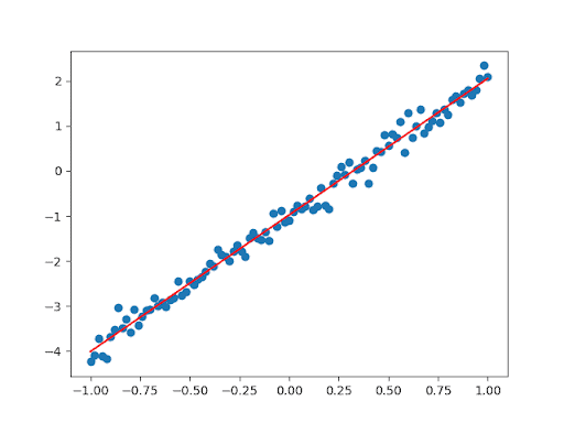
Let’s use our knowledge to code a trivial neural net in pure JAX. We want to implement a linear regression. Let’s create our data, a linear function plus some random noise:

n = 101

xx = jnp.linspace(-1, 1, n)

key_noise, key = jax.random.split(key)

yy = 3 * xx – 1 + 0.2 * jax.random.normal(key_noise, (n,))

Now we create a linear model with two parameters:

def model(params, x):

         return params[0] * x + params[1]

Note how the first argument (which we usually take a gradient over) is a pytree of the optimizable network parameters (just a size-2 list in this case).

Next, we define a loss function, compile it with jax.jit(), and calculate its gradient (with respect to params):

@jax.jit

def loss_fun(params, x, y):

         pred = model(params, x)

         return jnp.mean((y – pred) ** 2)

vgl = jax.value_and_grad(loss_fun)

Finally, we initialize the parameters and perform the training loop:

params = [1., 1.]

lr = 0.1

for i in range(100):

         loss, grad = vgl(params, xx, yy)

         params = jax.tree_multimap(lambda p, g: p – lr*g, params, grad)

         print(i, loss)

Note how we use jax.tree_multimap() to update our parameters (the vanilla SGD optimizer). The result looks like this:
OPTAX

This is going to be the shortest chapter of this article. In the previous example, we implemented vanilla SGD using jax.tree_multimap(). But we know it is better to use more advanced optimizers like Adam or SGD+momentum. Here, OPTAX comes to the rescue. Let’s see how we can modify the previous example using OPTAX. Since this is JAX, we must create an optimizer object (immutable, code-only) and then a state for it: 

params = [1., 1.]

lr = 0.1

optimizer = optax.adam(learning_rate=lr)   # Create the optimizer

opt_state = optimizer.init(params)        # Init optimizer state

Next, we rewrite the training loop by using the optimizer:

for i in range(100):

         loss, grad = vgl(params, xx, yy)

         upd, opt_state = optimizer.update(grad, opt_state)  # Optimizer step

         params = optax.apply_updates(params, upd)       # Basically params + upd

         print(i, loss)

First, the method optimizer.update() calculates the updates plus the new optimizer state. Second, we add the updates to the params using optax.apply_updates(), which is basically just a sum of two pytrees using jax.tree_multimap() under the hood.

Note that we use the same OPTAX optimizers regardless of whether our model is written in pure JAX, FLAX, or Haiku. Apart from optimizers, OPTAX also contains several loss functions and schedulers.

FLAX

FLAX: Basics

FLAX (FLexible JAX) is a layer API for JAX created by Google (DeepMind excluded). It plays a role similar to Keras in TF or torch.nn in PyTorch. We are going to use the modern flax.linen API, typically imported as nn; the old API flax.nn is deprecated and removed!

Let’s create a FLAX model of a single linear (aka FC aka Dense) layer:

model = nn.Dense(features=3)

This creates an (immutable) model object, but we also have to create and initialize the model parameters. For that, you need two things: a single-use random key key_init, and a sample input x (to specify input shape):

x = jnp.ones((4, 2))                            #  Sample input: batch_size=4, dim=2

key_init, key = jax.random.split(key)

params = model.init(key_init, x)     

Now, let’s print the parameter shapes:

print(‘params:’, jax.tree_map(lambda p: p.shape, params))

The output looks like this:

params: FrozenDict({

         params: {

                  bias: (3,),

                  kernel: (2, 3),

         }, })

What on earth is a “FrozenDict”? Basically, it’s an immutable python dict, defined in FLAX and registered with the JAX pytree ecosystem (which allows registering custom collection types). FLAX models prefer FrozenDict, but they can take python dict as well.

If the dictionary params consist of model parameters, why does it have a subdictionary named “params”? We’ll see it in a moment.

To run a model inference (or training) on a single input x, you type:

y = model.apply(params, x)

Note that you cannot use the parentheses operator! If the model requires a random key (e.g., for dropout), you’ll have to supply it as well:
y = model.apply(params, x, rngs={‘dropout’: key_do})

FLAX Models

But how can we create a FLAX model of more than one layer? There are several options. First, we can use sequential models (since FLAX 0.4.1):
model = nn.Sequential([

         nn.Dense(features=5),

         nn.relu,

         nn.Dense(features=3),

])

Note that nn.Dense() is a FLAX model object, while nn.relu is a function (with no parameters), nn.Sequential() supports both. 

For more serious models we’ll have to inherit the nn.Module class. Note that this class is a python dataclass (read about them if you didn’t already, they are fun):

class GoblinModel(nn.Module):

         feat1: int

         feat2: int


         def setup(self):                                  # This is called when init() is called

                  self.d1 = nn.Dense(self.feat1)       # A Submodule is registered

                  self.d2 = nn.Dense(self.feat2)


         def __call__(self, x):

                  x = jax.nn.relu(self.d1(x))             # Note: no apply(), no params !

                 return self.d2(x)

A dataclass defines several strictly-typed features (feat1, feat2 in our case) and automatically creates a constructor for them. That is why we should not define an explicit constructor in a dataclass, and the method setup() is used instead. It is called when you call the init() method of the model. Now we can create a model instance as usual followed by the initialization:
model = GoblinModel(5, 3)  # (feat1, feat2)

x = jnp.ones((4, 7))               #  Sample input: batch_size=4, dim=7

key_init, key = jax.random.split(key)

params = model.init(key_init, x)

A lot of magic happens under the hood when we call init(). It calls setup() and all submodules defined in setup() are registered, i.e. they are added to the parameter dictionary and initialized. Also init() handles random number keys under the hood and automatically generates a new single-use key for initializing each layer.

Note how in the __call__() method the submodules are called directly without giving them any parameters. When we run the inference, we actually call apply() and not __call__(), and the former method handles all parameters and passes all submodule parameters to the respective submodules.

However, the syntax with setup() is  somewhat cumbersome, thus people often use the decorator nn.compact() (a lot of black magic happens in this function) to define the submodules directly in __call__():

class OrcModel(nn.Module):

         feat1: int

         feat2: int


         @nn.compact

          def __call__(self, x):

                  x = nn.Dense(self.feat1)(x) # Layer    

                  x = jax.nn.relu(x)                # Function

                  return nn.Dense(self.feat2)(x)


A CNN example (CNNs are popular in computer vision) is not much harder:

class DwarfCNN(nn.Module):

         @nn.compact

         def __call__(self, x):

                  x = nn.Conv(features=32, kernel_size=(3, 3))(x)    # Layer

                  x = nn.relu(x)                                                         # Function

                  x = nn.avg_pool(x, window_shape=(2, 2), strides=(2, 2))

                  x = nn.Conv(features=64, kernel_size=(3, 3))(x)

                  x = nn.relu(x)

                  x = nn.avg_pool(x, window_shape=(2, 2), strides=(2, 2))

                  return x

FLAX models (custom layers)

So far, we created models out of standard FLAX layers. But how do we create a custom one? Here is an example. We use the method param() to define parameters:
class ElfLinear(nn.Module):

         feat: int

         w_init: typing.Callable = nn.initializers.lecun_normal()

         b_init: typing.Callable = nn.initializers.zeros


         @nn.compact

         def __call__(self, x):

                  w = self.param(‘w’, self.w_init, (x.shape[-1], self.feat))

                  b = self.param(‘b’, self.b_init, (self.feat,))

                  return x @ w + b

Due to the nn.compact() magic, we can declare the parameters directly in __call__() using the param() method. We need to supply an initializer and the shape. The latter is (in our example) derived from the input x, the sample input provided at the initialization. 

The Problem of State

But what if our model has a state (variables that are NOT trainable parameters)? For example, BatchNorm and related ..Norm layers have a state, and so do all models containing a BatchNorm as a submodule. This is where FLAX gets a bit awkward, in our opinion. We initialize the model as usual:

vars0 = model.init(key_init, x)

However, now the FrozenDict vars0 contain not only parameters (in the section params), but also state variables in other sections. Now we have to separate the two by hand:

state, params = vars0.pop(‘params’)

It is very important that the optimizer optimizes only parameters (params) and not vars0! In other words, we use params when initializing the optimizer and performing the optimizer updates. 

Before running apply(), we recombine parameters and state back into the dictionary vars, and use the form of apply() which updates the state. If we don’t want to update the state (a frozen BatchNorm at testing stage), we use the regular apply() instead:

vars = {‘params’: params, **state}

pred, state = model.apply(vars, x, mutable=state.keys())

Once again:

  • We must separate all model variables into state and param.
  • param (Network parameters) are optimized by the optimizer (via backprop).
  • state (Network state, e.g. batchnorm state) is updated in apply() during training, but is frozen during testing.

Do you think handling all the different parameters and states is awkward? We agree. However, for common training scenarios, FLAX provides a higher-level API FLAX TrainState, which combines model, parameters, and optimizer together. You can try it if you want. This is the highest possible level DL API, like fit() in Keras, or PyTorch Lightning.

Haiku

Haiku basics

Haiku is another layer API from DeepMind. Compared to FLAX, it is even purer functional programming. In FLAX, a lot of magic was buried in the nn.Module class and nn.compact() function. In contrast, in Haiku a model class does not matter. There is a class hk.Module, but it’s a thin submodule container that does almost nothing, and you don’t have to use it at all if you don’t want to. All elven magic happens in the function hk.transform() and its variations. Let’s see how it all works.

A neural net is always defined as a function (similar to the functional definition in Keras), for example:

def forward(x):

         return hk.Linear(3)(x)

Note that you define a Haiku module hk.Linear inside the function and do not provide any initialization data like input shape or a RNG key. Such a function will not work directly! Instead, you must transform it like this.

model = hk.transform(forward)

This step is similar to creating a functional Keras model (tf.keras.Model) in TensorFlow.

Now we get a transformed model object model. It works sort of like the FLAX module, but we never create such objects explicitly, only via hk.transform(). We still have to initialize it:

params = model.init(key_init, jnp.zeros((5, 2)))

Initialization is pretty much identical to the one in FLAX.

To run the model, we call apply():

y = model.apply(params, key_apply, x)

Note that in Haiku you must supply a RNG key in apply(), whether or not your model actually needs it (e.g., has dropout layers). If you want to get rid of this key, use an extra transformation:

model = hk.without_apply_rng(hk.transform(forward))

params = model.init(key_init, jnp.zeros((5, 2)))

y = model.apply(params, x)

A special version of hk.transform() is used when your model has a state (e.g. BatchNorm state):
model = hk.transform_with_state(forward)

params, state = model.init(key_init, x)                    # Init params + state

y, state = model.apply(params, state, key_apply, x)  # Apply model, update state

Only params are optimized. Note how Haiku separates params and state automatically, while in FLAX you had to do it by hand.

Haiku models

How do you define a model in Haiku? First, you can inherit hk.Module:

class GoblinMLP(hk.Module):

         def __init__(self, name=’goblin_mlp’):

                  super(GoblinMLP, self).__init__(name=name)

                  self.l1 = hk.Linear(5)

                  self.l2 = hk.Linear(3)


         def __call__(self, x):

                  x = jax.nn.relu(self.l1(x))

                 return self.l2(x)

You’ll still have to define a forward function (or lambda):

def forward(x):

         return GoblinMLP()(x)

But it’s Haiku, so you don’t have to use the model class if you don’t want to. How about this:

def forward_goblin(x):

         x = hk.Linear(5)(x)

         x = jax.nn.relu(x)

         return hk.Linear(3)(x)

It works, you can actually register layers in the forward function, without using the hk.Module class at all!

If you are writing a custom module, use hk.get_parameter() to register network parameters:

class GoblinLinear(hk.Module):

         def __init__(self, osize, name=’goblin_linear’):

                  super(GoblinLinear, self).__init__(name=name)

                  self.osize = osize


         def __call__(self, x):

                  n_in, n_out = x.shape[-1], self.osize

                  w_init = hk.initializers.TruncatedNormal(1. / np.sqrt(n_in))

                  w = hk.get_parameter(‘w’, shape=[n_in, n_out], dtype=x.dtype, init=w_init)

                  b = hk.get_parameter(‘b’, shape=[n_out], dtype=x.dtype, init=jnp.ones)

                  return jnp.dot(x, w) + b

You can even use parameters directly in forward(), without any hk.Module.

Haiku has a couple of further nice things. You can define an MLP (multi-layer dense network) concisely (it uses ReLU by default, this can be changed):
hk.nets.MLP([20, 20, 1])

There is also a number of standard architectures (but alas no pre-trained weights for them):

hk.nets.MobileNetV1

hk.nets.ResNet18, 34, 50, 101, 152, 200

So, Can JAX Succeed?

We don’t know it. But here are the good and bad sides of JAX, in our opinion (as compared to PyTorch and TensorFlow):

The good:

  • JAX is very TPU friendly and has built-in support for multiple devices.
  • Functional programming makes things a bit cleaner (but only for pros).
  • The weight of Google behind it should matter.

The bad:

  • It is still in the 0.x versions, the API might change.
  • Functional programming can be annoying for beginners.
  • Apart from the TPU, there are few real advantages over PyTorch (or TF).
  • There are very few deploy options. Currently, there is only the experimental jax2tf converter. No ONNX, tflite or TensorRT.
  • There is no dataset/dataloader API.
  • There are still very few existing or pre-trained models (but see flaxmodels).

Have fun and enjoy JAX! And if we you are more into video content, we have a lecture on JAX on our YouTube channel:

P.S. If the author were Google, he would create some nice deployment system for JAX, like tflite, but based on XLA, with versions for C++, Android, iOS, embedded and Web browser.

GStreamer C++ Tutorial

In the previous article, we’ve learned what GStreamer is and its most common use cases. Now, it’s time to start coding in C++. This tutorial does not replace but rather complements the official GStreamer tutorials. Here we focus on using appsrc and appsink for custom video (or audio) processing in the C++ code. In such situations, GStreamer is used mainly for encoding and decoding of various audio and video formats.

GStreamer C++ Basics

GStreamer C++ API is introduced rather well in the official tutorial, I’ll give only a very brief introduction before focusing on appsrc and appsink, the most important topic of interest to us. Our tutorial can be found here. In our code, we use C++, not C. Also, unlike the official tutorial, we are not too eager to use GLib functions like g_print().

Let’s get going. Our first example, fun1, is an (almost) minimal C++ GStreamer example. Before doing anything with GStreamer, we have to initialize it:

gst_init(&argc, &argv);

It loads the whole infrastructure like plugin registry and such. But why does it need pointers to argc, argv? You can put nullptr, nullptr if you really want to. But honestly providing your command line arguments allows gst_init() to parse GStreamer-specific flags. For example, I always add –gst-debug-level=2 to the command line in order to log warnings and errors to the console (there’s no logging by default). Interestingly, GStreamer removes all its flags from argc, argv, so that you can later parse the remaining arguments.

Next, we create a pipeline from a string

string pipelineStr = “videotestsrc pattern=0 ! videoconvert ! autovideosink”;

GError *err = nullptr;

GstElement *pipeline = gst_parse_launch(pipelineStr.c_str(), &err);

checkErr(err);

MY_ASSERT(pipeline);

Where MY_ASSERT is my assertion macro (like CV_ASSERT, never ever use the C++ assert statement !), and checkErr is my function that checks a GError object for errors, see the code for details. Checking for errors is important, to catch any typos in the pipeline string, linking failures etc. GStreamer is heavily based on GLib, especially on the GObject framework (a part of GLib), a pure C object-oriented framework. All GStreamer entities are GObject objects and they are handled as raw pointers. This may seem ugly compared to modern C++, but there is nothing I can do about it (as gstreamermm is now dead).

Now we created the pipeline, we should play it

MY_ASSERT(gst_element_set_state(pipeline, GST_STATE_PLAYING));

Is this all? Not yet. If we try to run the code at this point, it will simply run until the end of the main() function and shut down together with GStreamer, which didn’t even have time to start the pipeline properly. We must wait for the pipeline to finish. The simplest code for this is:

GstBus *bus = gst_element_get_bus (pipeline);

GstMessage *msg = gst_bus_timed_pop_filtered (bus, GST_CLOCK_TIME_NONE,

                           GstMessageType(GST_MESSAGE_ERROR | GST_MESSAGE_EOS));

gst_message_unref(msg);

gst_object_unref(bus);

GStreamer bus is a messaging system of a pipeline, which sends messages. Here we wait indefinitely for an error or end of stream (EOS), ignoring all other messages. Our further examples like fun2 demonstrate processing all messages in a loop, and eventually in a separate thread.

You might have asked: If our main() function is not blocked when the pipeline is running, then where does it run? In the other threads of course! GStreamer is multi-threaded and reasonably thread-safe (you can call the GStreamer function from different threads). There is NO such thing as GStreamer main loop. This can sound confusing, as many codes from the official tutorial use a GLib main loop. You absolutely don’t have to. The only point of this “main loop” is to block while watching the bus. As we watch the bus ourselves, we don’t need it. And it’s perfectly fine to use C++ threads with GStreamer, even though they didn’t exist when GStreamer was created (as they map into the same OS threads). GStreamer can also run several pipelines simultaneously if your PC is powerful enough for it.

Side note: The multi-threaded GStreamer philosophy is the opposite to the one of typical GUI libraries like Gtk+ or Qt, which run GUI strictly in a single thread with an event-processing main loop. GStreamer can be successfully combined with these libraries (see e.g. a Gtk+ example in the GStreamer tutorials), but this definitely goes beyond the scope of this article.

We are almost done with fun1. Now let’s exit the program cleanly by stopping and releasing the pipeline:

gst_element_set_state(pipeline, GST_STATE_NULL);

gst_object_unref(pipeline);

I remind you that C and C++ do not have proper garbage collection, thus memory leaks are always a big danger, often underestimated by people with backgrounds in other languages. And being a C library, GStreamer does not use nicer C++ features like shared_ptr, but has its own version of reference counting, thus “unref”. GStreamer memory management is confusing, and leaks are a persistent risk. The general rule is like this: if you don’t need myBanana anymore, try:

gst_banana_unref(myBanana);

If no such function, try

gst_object_unref(myBanana);

If the code does not work, then you shouldn’t unref myBanana for some reason.

This is it for the minimal example. It wasn’t very hard, was it? If you want to know more about GStreamer in C++, read the official tutorial and our other examples like fun2 and capinfo. There are tons of other things, like creating a pipeline programmatically (not from a string), dynamic and on-request pads, working with caps and pads, etc.

GStreamer C++ appsink and OpenCV Example (Video 1)

But what if we want to process each video frame in our own C++ code, not in some standard GStreamer elements? There are two ways to do this:

  • You can write your own element. This is hard for beginners, and I will not teach you this.
  • Use appsrc and appsink to move data back and forth between pipeline and our C++ code. This is what we will do.

We start with an appsink video example, video1. We want to decode a video file with GStreamer into raw data, and then visualize each frame with OpenCV’s imshow(). We’ll walk through the code briefly (see video1.cpp in our repo for details). The pipeline is given by the string:
filesrc location=<…> ! decodebin ! videoconvert ! appsink name=mysink max-buffers=2 sync=1 caps=video/x-raw,format=BGR
Wow, appsink has a lot of options! Let’s examine them all:

  • name=mysink : We have given our element a name so that we can find it.
  • caps=video/x-raw,format=BGR : Caps are vital. Here we specify that we want a BGR raw video signal. 
  • sync=1 : We synchronize the data to play at the 1x speed. Try sync=0 for fun! Note: true==1, false==0.
  • max-buffers=2 : Unlike most GStreamer elements, appsrc and appsink have their own queues. They can take a lot of RAM. This is an example of reducing the queue size. Only two frames are to be kept in memory, after that appsink basically tells the pipeline to wait, and it waits. Don’t try to reduce queues that much for branched pipelines!

If you need “global data” for a GStreamer pipeline it’s a good idea to create a structure for it, so that we will supply the data (as a pointer) to the callbacks if needed. In our case, all we need is the pipeline and the appsink element.

struct GoblinData {

GstElement *pipeline = nullptr;

GstElement *sinkVideo = nullptr;

};

We create an instance of this structure in main(), create the pipeline, and find the appsink by its name (“mysink”):

GoblinData data;
string pipeStr = “filesrc location=” + fileName + ” ! decodebin ! videoconvert ! appsink
    name=mysink max-buffers=2 sync=1 caps=video/x-raw,format=BGR”;

GError *err = nullptr;

data.pipeline = gst_parse_launch(pipeStr.c_str(), &err);

checkErr(err);

MY_ASSERT(data.pipeline);

data.sinkVideo = gst_bin_get_by_name(GST_BIN (data.pipeline), “mysink”);

MY_ASSERT(data.sinkVideo);

Next, we play the pipeline:

MY_ASSERT(gst_element_set_state(data.pipeline, GST_STATE_PLAYING));

Now, we have to wait for the bus, which we now put into a separate thread, see the code for details:

thread threadBus([&data]() -> void {

     codeThreadBus(data.pipeline, data, “GOBLIN”);

});

You can extract data from appsink by using either signals or direct C API, we chose the latter. We process data in a separate thread which we now start.
thread threadProcess([&data]() -> void {

     codeThreadProcessV(data);

});

Finally, we wait for the threads to finish and stop the pipeline:

threadBus.join();

threadProcess.join();

gst_element_set_state(data.pipeline, GST_STATE_NULL);

gst_object_unref(data.pipeline);

Everything interesting happens in the function codeThreadProcessV(). It has an endless loop for (;;) { … } , which we will eventually break out of. What’s in the loop?

First, we check for EOS:

if (gst_app_sink_is_eos(GST_APP_SINK(data.sinkVideo))) {

         cout << “EOS !” << endl;

         break;

}

Next we pull the sample (a kind of data packet) synchronously, waiting if needed. For raw video, a sample is one video frame:

GstSample *sample = gst_app_sink_pull_sample(GST_APP_SINK(data.sinkVideo));

if (sample == nullptr) {

         cout << “NO sample !” << endl;

         break;

}

Now, we want to know the frame size. It turns out, that the sample actually has caps (don’t confuse it with the pad caps), and we can find the frame size in there:

GstCaps *caps = gst_sample_get_caps(sample);

MY_ASSERT(caps != nullptr);

GstStructure *s = gst_caps_get_structure(caps, 0);

int imW, imH;

MY_ASSERT(gst_structure_get_int(s, “width”, &imW));

MY_ASSERT(gst_structure_get_int(s, “height”, &imH));

cout << “Sample: W = ” << imW << “, H = ” << imH << endl;

Next, we extract a buffer (a lower-level data packet) from the sample. Note: in GStreamer slang, a “buffer” always means a “data packet”, and never ever a “queue”!

GstBuffer *buffer = gst_sample_get_buffer(sample);

Still, we don’t have a pointer to the raw data. For that we need a map:

GstMapInfo m;

MY_ASSERT(gst_buffer_map(buffer, &m, GST_MAP_READ));

MY_ASSERT(m.size == imW * imH * 3);

Now we can finally read the raw data (BRG pixels) via the pointer m.data. But we want to process the frame in OpenCV, so we wrap it in a cv::Mat.

cv::Mat frame(imH, imW, CV_8UC3, (void *) m.data);

Warning! Such a cv::Mat object does not copy the data, so if you want cv::Mat to persist when the GStreamer data packet is no more, or if you want to modify it, then clone it. Here we don’t have to (but we DO clone in video3). Now we can do anything we want with the cv::Mat image, but in this example, we just display it on the screen:

cv::imshow(“frame”, frame);

int key = cv::waitKey(1);

Now, we release the sample, and check if the ESC key was pressed:

gst_buffer_unmap(buffer, &m);

gst_sample_unref(sample);

if (27 == key)

         exit(0);

We’re done with this frame, ready for the next one. In this example, we saw how to receive  GStreamer video frames from appsink, and convert them into OpenCV images via the sample -> buffer -> map -> raw pointer -> Mat route. 

GStreamer C++ appsrc and OpenCV Example (Video 2)

Now, the appsrc example, video2. Here we want to do the opposite to video1: read a frame from a video file with OpenCV’s VideoCapture and send it to the GStreamer pipeline to display on the screen with autovideosink. The pipeline is:

appsrc name=mysrc format=time caps=video/x-raw,format=BGR ! videoconvert ! autovideosink sync=1

The option format=time refers to timestamp format, NOT the image format from the caps! It is not required for video, but for some reason, it is required for audio appsrc, which will fail otherwise with rather obscure error messages (took me once a long time to figure this out).

This pipeline looks nice, but unfortunately, it will not work. If we try to play it, GStreamer will complain about the frame size. Indeed, we did not specify the frame size (width+height) in the appsrc caps, and it does not have a default one, so there is no way it can negotiate a frame size with the downstream pipeline. But we don’t know the frame size until we open the input file with OpenCV! How to solve this predicament? One could in principle defer creating the pipeline until we know the frame size, but it turns out that it is enough to defer playing it. This is exactly what we do in the function codeThreadSrcV(). In this function, we first open the input file with OpenCV and get the frame size and FPS:

VideoCapture video(data.fileName);

MY_ASSERT(video.isOpened());

int imW = (int) video.get(CAP_PROP_FRAME_WIDTH);

int imH = (int) video.get(CAP_PROP_FRAME_HEIGHT);

double fps = video.get(CAP_PROP_FPS);

MY_ASSERT(imW > 0 && imH > 0 && fps > 0);

Next, we create proper caps for our appsrc and set them with the  g_object_set():

ostringstream oss;

oss << “video/x-raw,format=BGR,width=” << imW << “,height=” << imH <<
          “,framerate=” << int(lround(fps)) << “/1”;

cout << “CAPS=” << oss.str() << endl;

GstCaps *capsVideo = gst_caps_from_string(oss.str().c_str());

g_object_set(data.srcVideo, “caps”, capsVideo, nullptr);

gst_caps_unref(capsVideo);

Now we can finally play the pipeline and start the infinite loop over frames:

MY_ASSERT(gst_element_set_state(data.pipeline, GST_STATE_PLAYING));
int frameCount = 0;

Mat frame;

for (;;) {

}

Inside the loop, we wait for the next frame from VideoCapture:

video.read(frame);

if (frame.empty())

         break;

We create a GStreamer buffer and copy the data there, again using the raw pointers frame.data and m.data:

int bufferSize = frame.cols * frame.rows * 3;

GstBuffer *buffer = gst_buffer_new_and_alloc(bufferSize);

GstMapInfo m;

gst_buffer_map(buffer, &m, GST_MAP_WRITE);

memcpy(m.data, frame.data, bufferSize);

gst_buffer_unmap(buffer, &m);

Now we have to set up the timestamp. This is important because otherwise GStreamer would not be able to play this video at the 1x speed:

buffer->pts = uint64_t(frameCount  / fps * GST_SECOND);

Finally, we “push” this buffer into our appsrc:

GstFlowReturn ret = gst_app_src_push_buffer(GST_APP_SRC(data.srcVideo), 
      buffer);

++frameCount;

Once we have exited the loop (upon the end-of-file), we want to shut down the pipeline gracefully by sending it an end-of-stream message.

gst_app_src_end_of_stream(GST_APP_SRC(data.srcVideo));

And now look at the code we described so far, and tell me: Is it good? It will run successfully if we start it, or at least seem to. But it has a serious flaw. Can you spot it? Pause for a moment and think carefully before reading any further.

You're thinking, right?

The answer is down below ⬇

Now, the answer. The VideoCapture decodes the video file as fast as it can, which can be quite fast on modern computers. However, our GStreamer pipeline is slow due to the sync=1 options (1x playback). But the pipeline will not signal our C++ code to slow down, the frame loop will run fast pushing more and more frames into the appsrc built-in queue, taking a lot of RAM, and possibly even crashing the application if the video is long enough.

This flaw (which is not obvious at all for beginners, by the way, did you guess it?) show how tricky designing pipelines (especially real-time ones) is, and how you should plan ahead and not code thoughtlessly. What is the solution? It’s obvious, we want the pipeline to signal when it wants data and when it doesn’t. Let’s register a couple of GLib-style signal callbacks on appsrc signals:

g_signal_connect(data.srcVideo, “need-data”, G_CALLBACK(startFeed), &data);

g_signal_connect(data.srcVideo, “enough-data”, G_CALLBACK(stopFeed), &data);

Since GLib is C and not C++, we cannot use lambdas or std::function in callbacks, only good old functional pointers. We supply the pointer &data to our data structure to make it usable by the callback functions. The callback functions simply set a single data flag:

static void startFeed(GstElement *source, guint size, GoblinData *data) {

using namespace std;

if (!data->flagRunV) {

     cout << “startFeed !” << endl;

     data->flagRunV = true;

}

}

static void stopFeed(GstElement *source, GoblinData *data) {

using namespace std;

if (data->flagRunV) {

     cout << “stopFeed !” << endl;

     data->flagRunV = false;

}

}

And now, we check this flag at the frame-processing loop and wait if the pipeline tells us to:

if (!data.flagRunV) {

         cout << “(wait)” << endl;

         this_thread::sleep_for(chrono::milliseconds(10));

         continue;

}

Beautiful, isn’t it? Now we learned how to use appsrc in addition to appsink and move the data both ways. While there is no direct connection between OpenCV classes and GStreamer (at least not without third-party plugins), we can easily move the data around using raw pointers and a few lines of code. Who needs the ready-made code, when you can write your own?

More GStreamer C++ appsink + appsrc + OpenCV Examples

My tutorial has a few more examples for you which I will list very briefly.

  • video3: This is like video1 and video2 combined. Here we have two pipelines, one with appsink (Goblin), the other one with appsrc (Elf) : We decode a video file with Goblin pipeline, process each frame with OpenCV, then send the frame to Elf pipeline to display it. This is the typical example of “decoding, then encoding with GStreamer”. 
  • audio1: The same with audio (no OpenCV in this code).
  • av1: The same with both audio and video.

Conclusion

In this series of articles, I have introduced GStreamer, explained why it is important, and then showed how it can be used for computer vision and audio processing. Enjoy GStreamer!