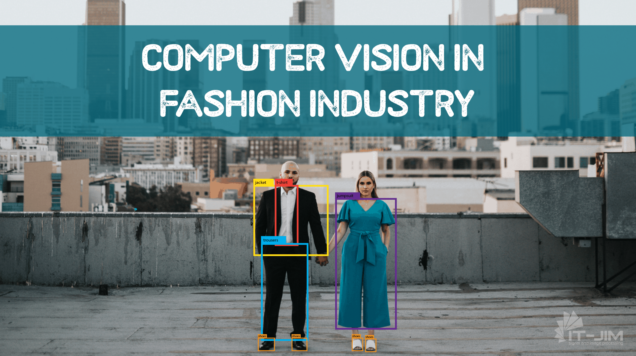
4 Ways How Computer Vision Is Deepening the Fashion Industry

What is your first thought when you hear about computer vision (CV) in fashion? Or, what is the first thing that pops into your head when you hear about deep learning fashion? Let us guess – online clothing shopping or virtual try-on applications?

Well, this might be surprising but deep fashion is not a far future anymore. What’s more, fashionably speaking, the usage of deep learning in the fashion industry seems to be already old-fashioned rather than pioneering or innovative. Many famous brands like Dior, Macy’s, Nike, Zara are already using artificial intelligence (AI) in e-commerce, and this is not only about market segments for retail clothing. There is far more than this within intelligent fashion. Most crucially, fashion is all about visuals. And where there are visuals, there is computer vision

Let’s see how exactly data analytics and AI approaches entered the fashion industry and what happens when so seemingly different fields come together.

As mentioned above, AI-powered tools have been already deeply embedded in many creative fields such as art, film, music, graphic design, advertising, and fashion. Being a multibillion-dollar global industry, fashion is what creates, sets, and sells style and image, and quite often dictates canons of beauty. 

Technically, making fashion truly intelligent is a very difficult task due to a huge variability of fashion items in style and design. Current trends on intelligent fashion are aimed at the tasks not only to detect clothing in an image but also analyze and synthesize new ones, and, hence, offer tailored recommendations. Within deep learning in the fashion industry, three main aspects appear definable: low-level pixel computation, mid-level fashion understanding, and high-level fashion analysis. The former is intended to label certain items on a picture and deals with human and cloth segmentation, landmark detection, and human pose estimation. Mid-level tasks aim to distinguish fashion images like items and styles. And finally, high-level analysis is recommendation-oriented, it includes synthesis and fashion trend forecast.

Here are the use-cases of how CV and deep learning are deepening fashion.

Try-before-You-Buy Solutions

An excellent example of CV-enabled fashion technologies is virtual fitting room applications. These allow potential customers to try on a garment or accessory using various software applications. You must admit it is great! Whether you choose glasses, watches, or hats, you are able to try on a model in real-time easily changing its color and shape.

Gap Dressing Room AR APP By Avametric – source

Such solutions are based on the pose estimation models used for landmarks detection. The deep fashion datasets might be taken from open-source libraries.

A yet harder task is to implement virtual try-on clothes. Because clothing alters its form when taking the shape of a person’s body, for proper augmented reality (AR) experience, a deep learning model should identify not only basic key points on the body’s joints but also the three-dimensional body shape.

Fashion Item Retrieval

Another benefit of using deep learning-based models is the fashion image retrieval task. For some, shopping can be enjoyable things to do, for others, could be absolutely frustrating. If you are not a shopping fan, when buying online can be even more challenging. You are just scrolling and scrolling, browsing gazillions of items, and could nohow find what you’re looking for. Or another case, imagine you saw a gorgeous Jennifer Lopez’s dress/purse/waistband (underline whichever is appropriate :)) and took fire to find something like that. Although many online retailer websites support keyword-based searches, it would be much handier if a mechanism existed which could help us to find the desired apparel based on a visual query rather than a text description alone. 

The great news is that CV may perfectly cope with this issue by finding a similar or alternative product you requested. And, most importantly, much faster than you would be searching by yourself. Still, clothing retrieval tasks based on queries by the customer’s picture is highly challenging. This is due to a significant discrepancy between the real-world photos and those captured by retailers. Another problem is that clothing items are highly deformable, and, thus, their appearance may differ dramatically.

To solve the clothing retrieval task there is a trend to create attribute-aware deep neural network architectures that may include both semantic attributes and visual similarity constraints into the feature learning stage. Some of them may exploit over-segmentation algorithms with human pose estimation to get query clothing items and to retrieve similar images from the existing galleries.

And here you can bring up a question: how does CV “know” what exactly should be retrieved?

How Computer Vision Understands Fashion

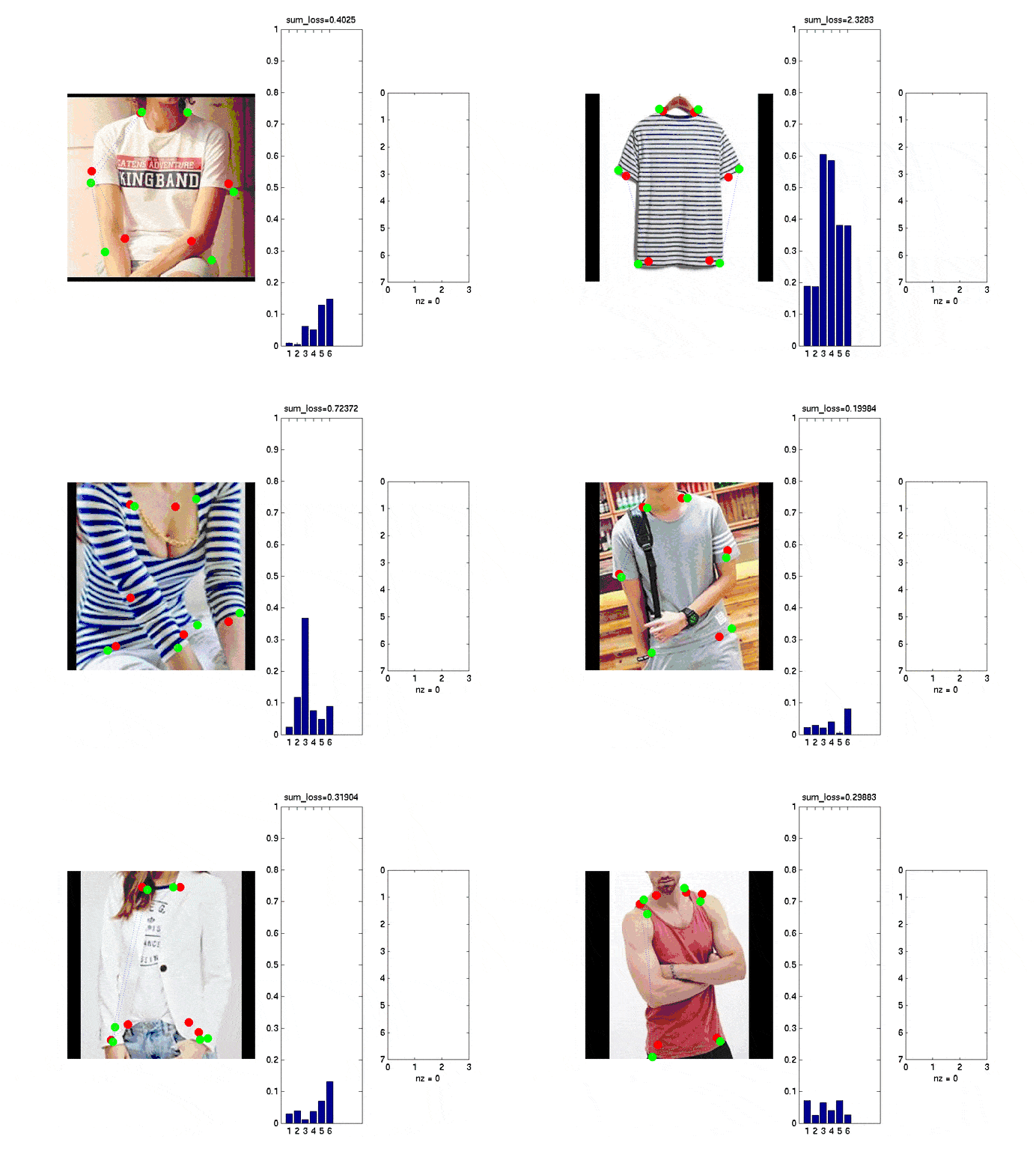
We know that CV systems are trained to “look” at the picture and generate a list of features for each detected item. This is mainly accomplished by such technology as landmark detection. The fashion landmark detection means recognition of clothing in an image and categorization of fashion items. Fashion landmarks are to define the precise location of such functional clothing regions as a neckline, hemline, sleeves and cuff. However, detecting fashion landmarks is a challenging task due to such constraints as background noise, human poses, and scales. For achieving more accurate landmark prediction, CV algorithms should be more context-aware. Besides that the landmarks indicate the key points on clothes, they also capture their bounding boxes, which helps better discriminate the design, pattern, and class of apparel.

An example of fashion landmark detection – source

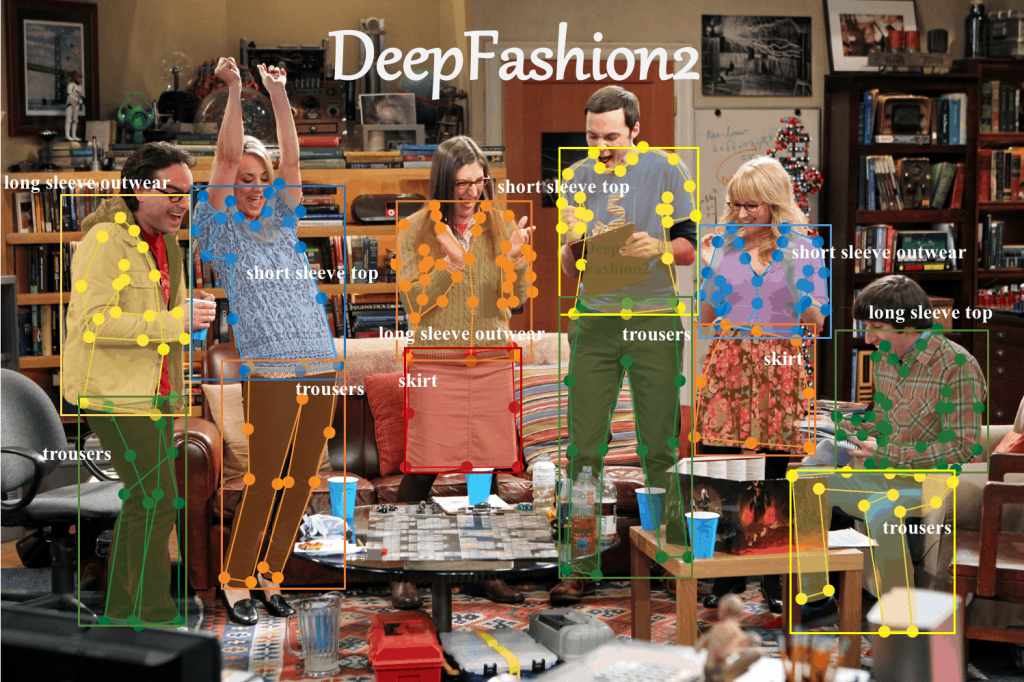
To be able to solve the above-mentioned tasks a number of clothes datasets come to the aid. One of the most widespread of them is Deepfashion2. It is a large-scale benchmark with comprehensive tasks and annotations, created by researchers from the Chinese University of Hong Kong. The dataset includes over 800K labeled into categories images with comprehensive descriptive attributes, bounding boxes, and clothing landmarks.

The Big Bang Theory series frame exemplifies the use-case of DeepFashion2 – source

DeepFashion2 allows performing a wide spectrum of tasks such as clothes detection, pose estimation, human and clothes segmentation, and clothing retrieval.

Fashion Recommendation with AI

A popular application of AI in clothing fashion is the deep learning recommendation engine. For e-commerce, it is all about categorization fashion items, clothing analysis, and help in certain style matching. Recommendation for fitting works on the concept of visual compatibility, which performs how favorable different fashion and apparel units can be matched to create a fashionable look. Also, it refers to the personalized recommendations considering such factors as preferable color, print, fabric, and outfit style. And since fashion is not only about what people are wearing but also reveals personality, fashion recommendation technology could help not only in certain cloth matching but in makeup or hairstyle suggestions. In other words, a customer benefits from the intelligent fashion-image consultant.

Another deep fashion application is a virtual assistant or chatbot. This kind of AI-powered software solution is an important part of business communication. Being an effective tool in user request analysis, it responds instantly and assists in keeping in touch with a customer throughout the whole purchase cycle.

Fashion Trends Forecasting Using Deep Learning

Given the frenetic pace in refreshment of fashion and design, retail businesses need to consistently keep up within the forefront and predict consumer preferences for the next season. Traditionally, such estimates are made based on the data from previous years. However, AI-based methods can reduce forecasting errors significantly. 

Besides obvious business interests in sales forecasting for the retail clothing market, it is also important for consumers to choose appropriate fashion goods. Deep learning models for fashion are impressively helpful in analyzing current trends and customers’ behavior. So, knowing what is and what expected to be on-trend, businesses can deliver a better brand experience and, thus, provide exactly what shoppers look for.

To sum up, today, AI methods provide multiple solutions for fashion making it more and more intelligent. CV-based deep fashion technologies come into use to handle diverse challenges, such as fashion image detection, item retrieval, analysis and synthesis, recommendation, and popularity prediction.

Computer Vision in Healthcare: Benefits & Key Applications

Computer Vision in Healthcare: Benefits, Challenges, and Use Cases

Are you interested in using new technologies such as  AI and computer vision in healthcare?

Artificial intelligence (AI) and machine learning (ML) are being increasingly used across various sectors, with healthcare being one of them. Computer vision (CV) technology is another powerful tool that helps recognize, interpret, and process visual data.

Computer vision in healthcare can transform existing patient care services by interpreting medical images and assisting in diagnostics with top accuracy. The potential applications of computer vision in the medical field are numerous, ranging from medical diagnostics and patient monitoring to treatment planning and automated health record management.

In this article, we examine the advantages of utilizing computer vision applications in healthcare and discover:

  • Understand computer vision in healthcare and how it works.
  • Reasons why computer vision matters in healthcare.
  • Ethical considerations in computer vision healthcare solutions.
  • Recent advancements in computer vision for healthcare applications.
  • Existing challenges in utilizing computer vision in healthcare.
  • Future scope and trends of computer vision in healthcare.

Let’s start by exploring what computer vision is and its impact on the medical field.

What Is Computer Vision and How Does It Work?

Computer vision, a subset of artificial intelligence (AI), empowers machines to interpret and understand visual data from the world around them. This technology aims to replicate human vision, enabling computers to perceive and process images and videos.

At its core, computer vision engineering focuses on key techniques like image recognition, object detection, and segmentation. These techniques help machines spot and categorize objects in an image, detect their boundaries, and segment different regions.

Computer algorithms learn from vast datasets, improving their accuracy and efficiency in tasks such as disease detection and medical image analysis. The use of a neural network further enhances these processes.

Why Does Computer Vision Matter in Healthcare

Experts cannot overstate the importance of computer vision in healthcare. The healthcare industry is embracing digital transformation, and integrating computer vision technology becomes essential.

AI-powered diagnostics enable healthcare providers to achieve unprecedented levels of precision, speed, and administrative relief. This allows not only to enhance efficiency but also to improve patient care and safety.

Global Market Insights estimated the global market for AI in computer vision at $14.1 billion. Analysts project that the market will grow at a 19.5% CAGR to $82.8 billion by 2034. This exponential growth reflects its critical role in the industry.

The need for more accurate and quicker analysis and healthcare operations drives this upward trend. Computer vision and AI systems are evolving and can now handle complex and varied visual data. This makes them a valuable tool in healthcare.

AI in computer vision market forecast

Additionally, computer vision techniques are revolutionizing the way researchers conduct medical image analysis. AI-driven systems analyze visual data with speed and precision. In contrast, traditional manual analysis is time-consuming and prone to errors. This not only enhances the diagnostic process but also frees up healthcare professionals to focus on direct patient care.

In addition to diagnostics, computer vision technology plays a crucial role in ensuring patient safety and quality of care. Computer vision enables automated remote monitoring systems that track patient conditions in real-time, as well as advanced computer-aided diagnosis, which aids in the early detection of diseases.

Medical professionals can now use computer vision to analyze complex images such as X-rays, MRIs, and CT scans. As a result, diagnostic errors are less likely to occur. This technology also helps ensure timely surgical interventions.

By implementing these innovations, healthcare organizations can improve patient monitoring, streamline workflows, and enhance the quality of care provided. 

The benefits of implementing computer vision in healthcare include:

  • Automate workflows, optimize resources, and speed up administrative tasks in a healthcare organization.
  • Deliver surgical assistance and improve precision and treatment outcomes.
  • Help detect anomalies in medical images and minimize diagnostic errors.
  • Enable continuous monitoring of patients (fall detection, movement tracking, condition changes).
  • Focus on patient care by handling routine tasks efficiently.
  • Interpret medical images accurately and effectively.
  • Enhance the user experience in healthcare environments.

Ethical Considerations in Computer Vision Healthcare Solutions

Ethical and privacy considerations play a crucial role in the implementation of computer vision in healthcare. Ethical considerations encompass data privacy and security, AI bias, and clinical validation.

Healthcare computer vision handles sensitive personal data, meaning it must meet industry standards and certifications. In a specific project case, consider these certifications and standards: FHIR, HIPAA, HITECH, CEHRT, ONC-ATCB, and GDPR.

EHR (electronic health records) certification builds trust among medical professionals, software developers, and patients. It ensures that the system uses data securely and adequately. EHR certification happens after a special executive board evaluates the software. For instance, in the USA, ONC and HHS are two organizations that handle this procedure.

Thus, to receive EHR certification, it is necessary to meet quality standards, mitigate the risks of unauthorized data access or hacking, establish robust data security protocols, and ensure top-notch data encryption and anonymization.

Transparency and accountability are also crucial for designing computer vision applications. Healthcare organizations must adopt transparent practices in data collection, processing, and training computer vision algorithms to ensure accurate and reliable results. Using practices that reduce bias in the training phase of deep learning models is essential for ensuring fairness and accuracy in AI-based applications.

To keep computer vision in healthcare private and secure, follow these criteria:

  • Robust software infrastructure with advanced security protocols and encryption.
  • Use of isolated servers, networks, and private cloud environments.
  • Centralized access control with unified authentication and zero-trust policies.
  • Autonomous systems that operate without human oversight.
  • On-device image processing that avoids transmitting or storing data in the cloud.
  • Local and real-time deep learning use (edge AI).
  • Transparent data handling and an easily understandable system architecture.

Fairness, transparency, and data security foster trust and encourage ethical use of computer vision technology in healthcare for everyone.

Key Applications of Computer Vision in Healthcare

The potential applications of computer vision in the medical field are multifaceted, ranging from image processing and predictive analysis to automated health record management. This improves the quality of medical services and the healthcare administration system.

Let’s consider computer vision use cases in healthcare today.

1. Computer Vision in Medical Imaging

Currently, the most widespread use of computer vision is image recognition and classification for medical purposes. AI-powered medical imaging can detect abnormalities in X-rays, MRIs, and CT scans faster than traditional analysis methods. Aided by CV and deep learning tools, physicians can inspect and interpret images in-depth, improving the accuracy of diagnosis and adjusting therapy accordingly.

Thus, medical image classification using a convolutional neural network (CNN) is employed to aid in disease diagnosis and treatment. Dealing with MRIs, for example, various CNN architectures may reveal tumors or aneurysms in the brain, and even predict the development of Alzheimer’s disease in the early stages.

Another way to use CV in medical imaging is through facial recognition and video stream processing. One of the benefits is that deep learning algorithms can be successfully trained to reveal even the slightest abnormalities. This aspect could be extremely helpful for patients suspected of developing conditions and rare genetic malfunctions that are difficult to detect in routine screenings.

Several computer vision healthcare companies have developed AI face-scanning applications. Based on ML algorithms and neural networks, they classify distinctive features in photos of patients with congenital and neurodevelopmental disorders.

2. Computer Vision for Surgical Assistance

Computer vision systems also have a great application in surgery. In this field, computer vision is a powerful tool for enhancing surgeon performance by measuring activity levels, detecting chaotic movements, and assessing working times in particular areas – ROI (regions of interest).

The technology enables training and simulation, as well as assessing surgical skills to enhance surgeon performance. This way, medical personnel can effectively prepare for invasive surgical procedures while minimizing potential complications.

Additionally, computer-aided models can accurately reconstruct surfaces and design implants for orthopedic procedures. This CV application can provide prompt and precise segmentation of bones, joints, or soft body tissues. This helps achieve higher levels of accuracy in modeling skeletons and implants for surgeries, taking into account the MRI and CT scans.

Another notable example of a deep learning system for surgical assistance is the Triton project. The system estimates real-time blood loss during and after surgery by visually analyzing blood-soaked sponges, suction containers, and other surgical tools. This tool helps determine the appropriate amount of blood to transfuse during or after the procedure.

3. Computer Vision in Early Disease Detection

Early disease detection is crucial for enhancing patient survival rates and simplifying their treatment. AI-powered systems are trained on a large volume of medical imaging data, allowing for the identification of patterns and anomalies that may not be visible to the human eye. This capability is particularly significant for conditions like lung cancer, where early detection can lead to more effective treatment and a more favorable prognosis.

Additionally, mobile devices equipped with convolutional neural networks can facilitate early diagnosis in dermatology, allowing patients to monitor their skin health more easily. This feature aids in skin cancer detection by analyzing images of skin lesions, enabling timely intervention and reducing the risk of skin cancer progression. 

Similarly, AI-driven screening tools enhance preventive care by identifying patients at high risk. These tools are handy to diagnose diseases such as Alzheimer’s disease, cardiovascular disorders, and diabetic retinopathy.

4. Tumor and Cancer Detection with CV

One of the most significant applications of computer vision in healthcare is the detection and segmentation of tumors. Deep learning technologies have significantly enhanced the accuracy of detecting those, allowing for earlier cancer diagnosis and treatment.

Segmentation techniques such as Mask R-CNN are used to provide accurate and detailed outlines of tumors or melanomas. This automation streamlines the detection process, making it less time-consuming and tedious, and allowing radiologists to focus on their vital tasks. 

Moreover, deep learning models have achieved physician-level accuracy in cancer detection, highlighting the potential of computer vision to augment human expertise. For instance, a recent study on breast cancer reveals the successful application of AI and deep learning methods, achieving a model accuracy of 97.18%.

Another key aspect of tumor detection is characterizing tumors based on their morphologically relevant features, such as roundness and aspect ratio. These features help in analyzing the shape and structure of tumors, leading to more accurate diagnoses and personalized treatment plans.

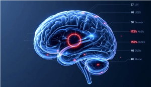
An example of medical imaging enhanced by computer vision techniques, demonstrating tumor detection.

5. Automated Health Monitoring with Computer Vision

Another example of a successful CV application is the real-time tracking of vital signs and fitness characteristics. This application can prevent acute neurological and cardiac events, such as strokes and heart attacks.

Computer vision has shown promise in remote patient monitoring, enhancing care for chronic conditions and post-surgery, particularly among elderly individuals. Additionally, by utilizing AI-driven technology, personnel can make clinical decisions more quickly for emergency care prioritization and optimal timing for surgeries.

6. Infection Prevention & Control of Pandemics

Artificial intelligence and deep learning solutions can become a valuable method for controlling and preventing pandemics.

For instance, the open-source community COVID-Net was the first to develop a convolutional neural network for detecting coronavirus cases from CXR images. It is possible to reveal the infected part of the lungs and diagnose COVID-19 with 92.4% accuracy.

The research is available to the general public to design a highly accurate and practical solution for detecting COVID-19 cases and improving treatment plans.

Thus, CV imaging data helps prevent disease spread by detecting masked faces, screening for germs, and using thermography to reveal temperature differences in a body or object.

7. Hygiene Compliance at Hospital with CV

Computer vision is a powerful tool for maintaining hospital hygiene and ensuring compliance with safety protocols. Automating the inspection of patient rooms and surfaces can detect dust, dirt, and other contaminants that pose health risks to both patients and medical staff. Utilizing artificial intelligence and deep learning, these systems assess surfaces for cleanliness, monitor disinfection activities, and pinpoint areas that require attention.

Computer vision can also track human behavior. It can detect if hospital staff forget to sanitize their hands or if visitors enter restricted areas without proper protective gear. By automating these checks, hospitals can respond quickly to hygiene lapses and enhance overall patient safety.

8. Healthcare Research & Drug Discovery

Computer vision can serve as a valuable tool for interpreting complex medical imaging and making more informed decisions.

CV algorithms can monitor patients participating in clinical trials. When integrated with electronic health records (EHRs), it enables seamless access to patient data and promotes effective collaboration across multidisciplinary healthcare teams.

This system enhances patient selection, recruitment, and retention throughout the trial process. It also helps reduce the overall cost of clinical trials and accelerates the FDA approval timeline for new drug therapies.

The technology also has its application in new medicine development. Creating a new drug is a highly time-consuming, complex, and costly process, and takes around 10-15 years. Failures are common and carry significant financial consequences. AI-driven drug discovery offers an innovative approach that may save time and financial resources in the development of new medicines.

9. Computer Vision for Enhancing Administrative Processes

Finally, by utilizing a CV in the healthcare system, numerous manual administrative processes can be easily automated. Among them are patients’ health records that should be reviewed and updated by doctors, protocol recordings, insurance documentations, and similar.

Another benefit of computer vision in healthcare is the reduction in workload. Traditional image analysis is time-consuming and labor-intensive. However, computer vision applications can optimize this process, enabling medical workers to focus on more complex cases. 

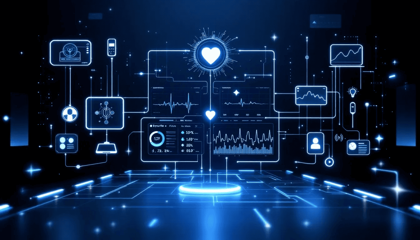
A graphic illustrating the importance of computer vision in healthcare, highlighting its benefits for patient safety and diagnostics.

Computer vision technology enhances the efficiency and accuracy of healthcare workflows, significantly reduces costs, and improves patient care and treatment outcomes.

Radiology, cardiology, dermatology, orthopedics, ophthalmology, telemedicine, and pharmaceutical research are the primary application areas. On the other hand, computer vision technology for healthcare systems may assist in multiple areas:

  • Provide more accurate diagnosis and health monitoring.
  • Develop personalized medicine.
  • Detect illnesses and conditions that are difficult to identify.
  • Create infrastructure for future research and clinical trials.
  • Enhance decision-making and support the prescription of appropriate treatment.
  • Optimize medical administrative tasks (generating automated protocols and reports).

CV Applications in Healthcare: Technical Challenges and Limitations

While the potential of computer vision in healthcare is immense, several technical challenges and limitations must be addressed.

CV and image processing can encounter failures when devices malfunction due to software bugs or viruses. Additionally, differences in an object’s size, angle, or distance from the camera can impact how it appears, causing distortions and inconsistent recognition.

Here we’ll outline the key challenges associated with applying computer vision in healthcare settings.

1. Data Privacy and HIPAA Compliance

Data privacy is one of the primary barriers to integrating deep learning algorithms. Healthcare datasets contain the most sensitive information, making it crucial to implement secure frameworks and infrastructure that comply with HIPAA or similar regulations.

Overcoming these obstacles and ensuring that patient data is secured and protected against unauthorized access opens up numerous possibilities for utilizing artificial intelligence.

2. The Need for Datasets to Train AI Models

A significant amount of healthcare data is necessary to train computer vision and deep learning systems. Healthcare computer vision requires datasets with accurate annotations of medical imaging, which can be challenging to obtain due to the diversity, privacy, and sensitivity of healthcare data.

Only when sufficient high-quality data is available is it possible to develop a robust AI-based system that recognizes patterns and abnormalities. Bias in training data is also a significant challenge for data scientists. Computer vision algorithms can hold existing biases if the training data is not diverse and representative of the population.

Thus, all healthcare entities should unite forces to collect, assemble, and unify anonymized datasets that contain information on health conditions and various demographics, thereby improving model accuracy.

3. Integration with Legacy Medical Systems

Integration with legacy systems presents another barrier to the broader adoption of healthcare computer vision. Many healthcare organizations rely on established systems that may not be compatible with new AI-driven solutions.

Overcoming these integration challenges often requires a step-by-step approach tailored to cover the needs of existing systems within a healthcare setting. Additionally, it is essential to offer post-launch employee training programs to optimize the benefits of artificial intelligence utilization.

To conclude, another significant obstacle to CV and digital health is the lack of AI and ML professionals with the necessary practical experience and knowledge to ensure the systems function properly and fully utilize computer vision systems.

Future Scope of Computer Vision in Healthcare 

The primary goal of computer vision in healthcare is to develop systems that can understand, interpret data, and act in a manner similar to humans in the medical domain. 

CV technology can help doctors analyze health vitals and fitness measures for more informed, precise, and quicker diagnosis. For instance, AI-powered software can convert images into interactive 3D models to aid in evaluating health conditions and diagnoses.

A futuristic depiction of computer vision applications in healthcare, showcasing potential advancements.

These are a few aspects that define the evolution of CV technology in healthcare:

  • The manufacturing of more powerful graphics processors and video adapters continues to increase processing power, enabling real-time image classification and recognition to occur significantly faster.
  • A growing number and quality of health databases, combined with the advancement of deep learning algorithms, will further facilitate the development of CV-enabled applications with higher accuracy and a greater level of detail.
  • More CV-enabled apps will move to the edge, meaning that the solution will operate locally, on terminal devices. This way, apps can deliver instant replies to medical image analysis, eliminating the need to wait for cloud data processing.
  • Convolutional neural networks and machine learning algorithms provide automated, accurate medical image analysis and reporting. This results in considerable time savings, output maximization, and the removal of human mistakes.

Also, regulatory acceptance of AI/ML technologies is growing. The FDA has approved numerous AI/ML-enabled medical devices, indicating a wider adoption of computer vision technologies in the healthcare domain.

To conclude, the future of computer vision in healthcare appears promising and is poised to play a significant role in transforming the industry. Artificial intelligence, machine learning, and computer vision are advancing patient care, diagnostics, and treatment.

Concluding Thoughts on Computer Vision Technology in Healthcare

The journey towards a more advanced and efficient healthcare system is just beginning, and computer vision is at the forefront of this exciting transformation. 

The availability of large digital data volumes plays a crucial role in leveraging CV-based software in healthcare. This factor ensures high-quality medical services and an optimized administration system. 

Computer vision in healthcare is revolutionizing by enhancing diagnostics, patient monitoring, surgical assistance, and pathology analysis. The technology improves patient care and treatment, laying the foundation for a more efficient and accurate healthcare system.

To summarize, the computer vision for healthcare systems may assist in:

  • Providing more accurate diagnoses and health monitoring.
  • Developing personalized treatments and medicine.
  • Detecting diseases and health conditions that may be difficult to find in early stages.
  • Creating infrastructure for future research and clinical trials.
  • Enhancing decision-making and facilitating the prescription of appropriate treatment.
  • Optimizing medical administrative tasks.

At It-Jim, we invite you to explore how computer vision can enhance your healthcare practice. We can help with a custom CV and AI solution development, meeting your requirements. By embracing these technologies, you can achieve better care quality, enhance patient safety, and deliver improved patient outcomes.

Let’s build the project together and explore opportunities to integrate the latest technologies.

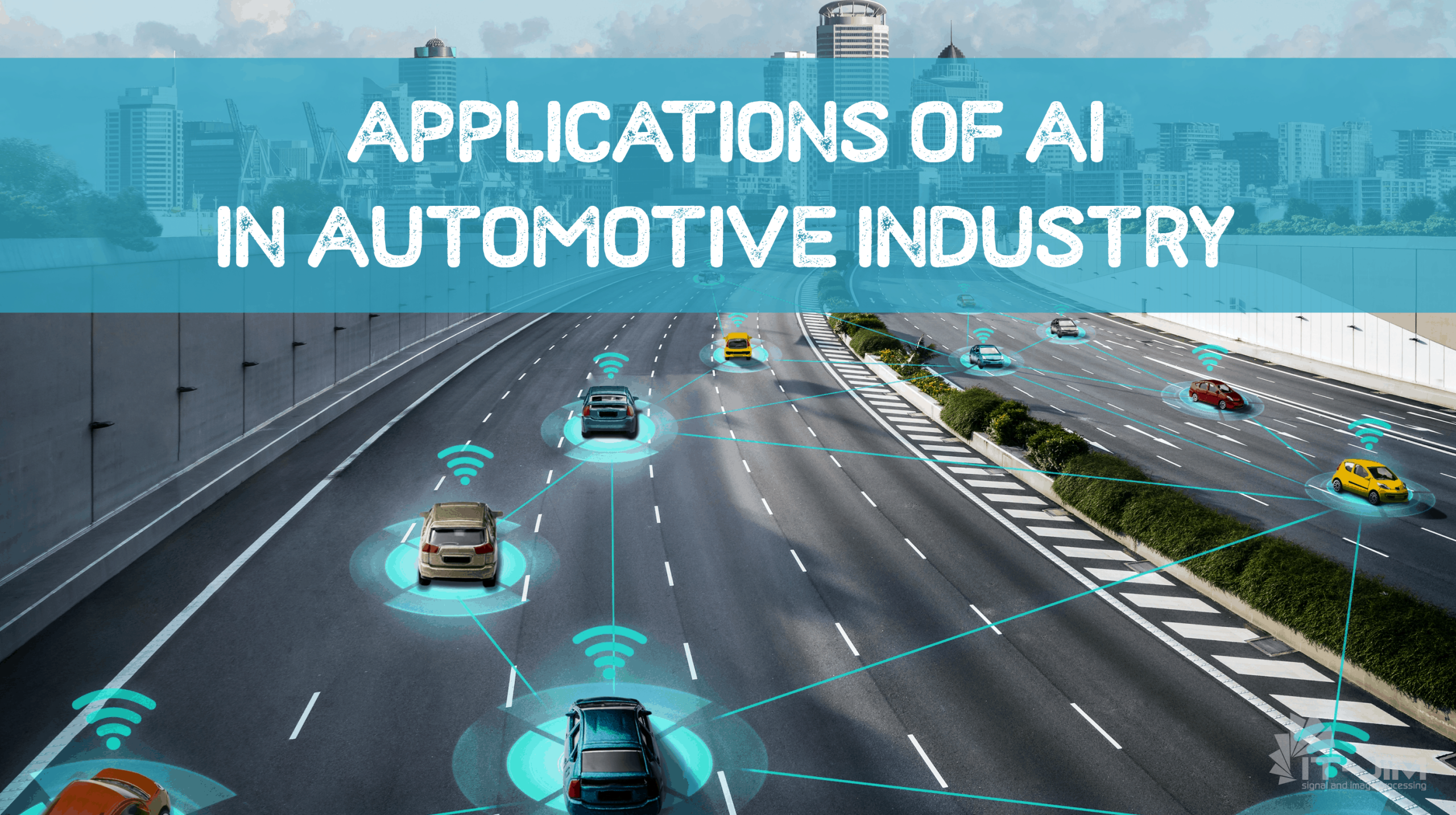
Applications of Artificial Intelligence in Automotive Industry

A century ago, the very thought of machines being able to think, make complicated calculations, and come up with effective solutions to pressing problems was more of a figment of science fiction writer’s fantasy rather than a foreseeable reality. Still, as we move into the third decade of the 21st century, we cannot imagine our life without manufacturing robots, marketing and stock trading bots, virtual travel agents, smart assistance, and other things that wouldn’t have come into existence without the achievements in artificial intelligence and machine learning. The role of artificial intelligence and machine learning in the automotive industry is also difficult to underestimate. According to recent reports, the global automotive AI market is poised to grow to $15 billion within the next five years, and for good reason. With AI driving bringing more applications to the automotive industry, more companies decide to deploy AI and machine learning models in the production environment. In today’s article, we’re going to take a closer look at the ways artificial intelligence is transforming the automotive industry and serves its current needs.

A Few Words about Artificial Intelligence

Want to learn more about artificial learning and deep learning in the automotive industry? Let’s first take a closer look at the definitions and main objectives of these branches of computer science. 

Artificial Intelligence science along with its well-known machine learning and deep learning branches pursue concrete goals, which can be inferred from its very name. AI aims to enable machines to carry out the functions and complete the tasks which are normally performed by humans. In essence, AI is a machine with the ability to solve problems hitherto solved by us, humans with our natural intelligence. To evolve to strong AI machines need to learn. When machines can extract meaningful conclusions from large volumes of data sets, they start to demonstrate the ability to learn deeply. Deep learning requires artificial neural networks that operate similarly to biological neural networks in humans. The three technologies now help scientists and analysts interpret tons of data and are hence indispensable for the field of data science. And now it’s high time we discussed the significance of artificial intelligence and data science in the automotive industry.    

Artificial Intelligence and Production of Vehicles

AI is having a large impact upon the automotive sector. We see AI as part of Industry 4.0 initiatives driving up efficiencies in manufacturing plants by improving overall equipment effectiveness, reducing defects, and improving automation on the line. AI is a value-add to data. This means that the manufacturer needs to have a good data environment or a route to a good data environment. Most of the data collection software installed in the last 20 years will have a good set of sensors on them. The collection of data, as well as data science applications in the automotive industry, is extremely important from a holistic point of view. Presently, lots of companies that provide AI services enable automotive businesses to improve their data environment to reach the state where they can leverage AI and realize the value from their data. The automotive sector can also benefit from good AI solutions capable of acting in advance of real time. This can help companies reduce costing, shipment, and robotic weld defects significantly. Automating visual inspection with the help of AI can in turn go a long way in reducing human error in the process and improve traceability. 

Self Driving Cars

When speaking of automotive machine learning projects, it’s impossible not to mention self-driving car solutions. Major technology companies like Lift and Waymo, as well as the automakers like Toyota and General Motors, have spent billions of dollars developing self-driving cars. Autonomous buses and shuttles are currently being deployed in cities and airports, driverless trucks are already delivering goods long distances, and even autonomous flying taxis seem to be our near future. And there’s a good reason for this rapid integration of machine learning in the automotive industry

First of all, self-driving cars will greatly reduce transportation costs for consumers. And by using autonomous fleets of shared electric cars we’d only need ten percent of cars on the road currently, which can help to significantly reduce CO2 emissions. When that shift happens, people will be able to redesign cities and create a safer environment for everyone. The data from the National Highway Traffic Safety Administration indicate that more than 90 percent of car accidents are caused by human error. This means self-driving cars have the potential to save more lives than airbags, seat belts, and stability control combined. 

Although implementing ML in the automobile industry is an expensive technology, there’s definitely room for startups in this space that can create software and collect data needed to scale autonomous vehicles globally. They aim to make these cars safer by gathering data from human drivers. And there’s a big space to combine blockchain technology with fleets of these cars to create even more autonomous systems which Porsche has started trying out to increase the transparency of the decisions made by driverless cars. 

Lots of people wonder how driverless cars can recognize potential threats and react to the environment in real time. Probably, you’ve heard of self-driving cars using neural networks, specific algorithms that power autonomous vehicle perception. Exactly these neural networks enable driverless vehicles to orient themselves on the street and avoid collisions.   

  • Computer Vision

Self-driving vehicles have five core components that help them navigate and maneuver through street traffic. Computer vision is the first step in that pipeline. Whereas humans rely on eyes and brain to handle the steering wheel, whereas out driverless counterparts take advantage of computer vision. Driverless cars use computer images to find lane lines and track other vehicles on the road. The majority of autonomous vehicles utilize lots of cameras to monitor the environment in the most effective way. Tesla, for example, equips its cars with eight surround cameras that provide 360-degree visibility of the area about 490 feet around the car. There are so many tasks that cameras enable, like lane finding, road curvature estimator, obstacle detection, stop sign classification, traffic light detection, and much more. 

  • Sensor Fusion 

Now that we’ve learned so much about computer vision in the automotive industry, it’s about time we took a look at other components. As good as cameras are, there are certain measurements like distance and velocity at which other sensors excel. And some sensors can work better in adverse weather. By combining all other sensor data, we get a better understanding of the world. There are different sensors for different use cases. Thus, radar is good for determining how far away the object and how fast it’s going. Lidar, in its turn, emits an array of laser beans creating a 3D-point cloud and serves as an effective media between a camera and radar. Ultrasonic sensors, on the other hand, have a small sensing distance which makes them useful for lateral movements like parking. 

  • Localization

Localization is how driverless cars figure out what their position in the world is. Our phones are equipped with GPS, so they help us orient ourselves in the unfamiliar terrain. For cars, more sophisticated algorithms are used, though. They help a car localize itself in a given map with the accuracy of 3, 93 inches by matching the point cloud it sees to the point cloud that the map has. 

  • Path Planning

The car charts a trajectory through the world to get to where it wants to go. First, it needs to predict what the other vehicles around it will do to decide which maneuver to take in response to the situation. Lastly, the trajectory is built to execute the maneuver safely. 

  • Control 

Once the car has a trajectory, it has to turn the steering wheel and hit the throttle or brake accordingly to follow that trajectory. When we have an idea of the path we want our cars to follow, we try to control it. At times, controlling a vehicle can be quite tricky, like attempting a hard turn at high speed. This is something race car drivers are good at, and computers now try their best not to fall behind. 

With more industries acknowledging the importance of AI, more self-driving car projects using machine learning are being created on a daily basis. It’s a rare person who would deny the fact that artificial intelligence in car systems is a perfect tool for more than making machines smarter and predicting their failures and malfunctions. Even though challenges still exist, different fields within the automotive industry are already harnessing the potential of the aforementioned techs and seeing increased efficiency and optimization of processes. 

Real-Time Video Pipelines: Techniques & Best Practices

Practical Guide to Real-Time Video Pipelines: Tools, Techniques & Optimization

Video is an extremely popular way to represent information. Indeed, sometimes, it is enough to watch a short clip instead of listening to a podcast or reading about complicated technical concepts.

Businesses also strive to gain a competitive advantage by integrating innovations like video analytics, streaming services, robotics, and AR/VR apps. To get valuable insights from raw video data, you need to design and implement efficient video pipelines.

From a user’s point of view, a video is simply a sequence of images displayed one after another with a very short inter-frame interval. Typically, it has around 30 frames per second (FPS). However, many things are left inside the box.

In this article, we focus on how to build an efficient video streaming pipeline and explore:

  • What is a video pipeline from a technical perspective.
  • Essential elements of video pipelines.
  • Ways to design and develop efficient video pipelines.
  • Share our It-Jim experience and best practices for building a video pipeline.
  • Tools, frameworks, and technologies for building video pipelines.

Let’s explore what a video pipeline means and how it is utilized in computer vision, compared to traditional image processing methods.

Understanding Video Pipelines

So, what is a video pipeline?

At its core, a video pipeline is a sequence of processing steps that takes raw video from cameras or sensors and turns it into output or actionable insight for the end user. This technology is used in computer vision systems for object detection, tracking, and monitoring.

The primary goal for developers is to maintain high video quality while optimizing storage, scalability, and seamless playback across various devices and networks.

The main components of a video pipeline are input sources, transcoding servers, content delivery networks (CDNs), and processing tools. Once these video pipeline components are aligned to work together, the system delivers a smooth viewing experience and is a reliable analytics tool.

Traditional image processing works with single, static images. There’s no pressure to process them quickly, so it’s often done offline without time constraints.

In contrast, video processing pipelines work with a stream of frames. Each frame arrives in rapid succession and is connected to the ones before and after it. For many use cases, such as live streaming, surveillance, or AR/VR, each frame must be processed in real-time or near real-time to ensure smooth playback and timely analysis.

Real-time pipelines differ from non-real-time ones in that they are designed to operate with minimal delay, often under hardware constraints. Real-time video pipelines process frames as they arrive, prioritizing low latency and smooth playback for live applications.

Non-real-time pipelines handle pre-recorded video, allowing slower, more complex processing without time constraints. Both types share the same components but differ mainly in timing and performance requirements.

In summary, either system requires a real or non-real-time video pipeline setup; the process can be complex and costly. Next, we will outline the key aspects of its careful planning and implementation.

How Video Pipelines Work

A video pipeline consists of several phases, including capture, processing, and encoding. Here is the workflow of a standard video pipeline:

  • Capture raw video through a camera.
  • Process the video (apply filters, AI models, or CV algorithms).
  • Encode it for storage or streaming.
  • Repackage frames for storage or transmission.
  • Deliver output to the user or system.

The first steps in a video pipeline are capturing raw video, uploading it to a server or cloud storage, and extracting metadata from the original video.

Whether you’re building a smart surveillance system, a robotics platform, or a live video analytics service, your video pipeline has a direct impact on the accuracy and performance of your solution.

Key Components of Video Pipelines

The main components of a video pipeline are video sources, transcoding servers, Content Delivery Networks (CDNs), and various processing tools.

Thus, most of the video pipeline consists of the following:

  • Video sources – these can include a camera, video files, or a live stream.
  • Encoding and decoding – the process of converting video into different formats for storage and transmission.
  • Transcoding – convert video from one format to another, also for different platforms or devices.
  • CDN integration – distribute video content through a network of servers to reach users faster.
  • Display elements – prepare the video for playback on various devices (e.g., TVs, computers, mobile phones).

A well-tuned video pipeline seamlessly integrates all its video pipeline components. A good understanding and implementation of the components can make a big difference to the efficiency and reliability of your video pipeline.

Next, you can check out an example with code samples on how to build a video pipeline.

Building Efficient Real-Time Video Pipelines

Have you ever written your own video player? What about a media server? Or a real-time video processing pipeline?

For most people in the world, the answer is “no”. Probably even among the readers of this blog.

Our experience suggests that many people underestimate the difficulties involved and are in for unpleasant surprises when attempting to implement computer vision (CV) in real-time.

 “Real-time” refers to the process of receiving frames from a camera or network stream, as opposed to a pre-recorded video file.

Novice computer vision engineers typically learn their craft on individual images. In rare cases, when the time dimension is required (e.g., tracking, optical flow), they usually work on pre-recorded videos.

Then they think: What can go wrong with real-time? I just get frames from the camera and apply the fancy computer vision that I usually do?

A schematic C++ code they imagine looks like this:

cv::VideoCapture cap(cv::CAP_ANY);
while (true) {
cv::Mat frame;
cap.read(frame);
process_somehow(frame);
send_somewhere(frame);
}

Is it how a good real-time computer vision system works? No! Let’s dive deeper.

Where is the Frame Loss?

When junior CV engineers try to do something with a camera, our first question is, “Where is the frame loss here?”

This question usually surprises people: “No, I do not want to lose any frames”. This is wrong. If your camera produces 30 FPS, few CV algorithms (and especially not neural networks) can process a frame in 33 milliseconds.

Then, you typically want to stream, display on screen, or record the result somewhere. This also takes time. Even if your computer is fast enough, there are always slower devices (such as embedded ones) or computers overloaded with some background tasks.

So, frame loss is inevitable. And because of the frame loss, you can never rely on a steady FPS from a camera.

Pop Quiz: Where is the frame loss in the piece of code above? Think before reading the answer.

Now, here is the answer: the frame loss is at the line “cap.read(frame);”. This is a synchronous waiting call “give me the next frame when ready”. If you take too long processing frame 1, the subsequent frames will be lost until you reach the read() call again.

Luckily for us, OpenCV VideoCapture does not try to keep multiple frames in a buffer. You can guess what would happen if it did.

Hint: Nothing good.

Again, frame loss means that there is no reliable fixed frame rate (FPS) and that the difference between the timestamps of two subsequent frames varies.

It does not matter if your CV algorithms process each frame individually. It is usually not critical for optical flow either.

However, if you perform signal processing in the time domain or use parameterized motion models, then frame loss becomes critical.

What is the solution?

You must record the original timestamp of each frame. If you need a signal with a regular frame rate (FPS), resample the original video to a desired regular timestamp grid.

Threads and Buffers to the Rescue

Does the code above work correctly? Yes. Is it efficient? Definitely not.

Note how it does all operations strictly sequentially. This includes an input (get a frame from the camera) and output (visualize the result on the screen, write it to a file, or send it to the network).

Such a sequential pipeline does not utilize (or at least does not utilize efficiently) multithreading on multiple CPU cores (and possibly a GPU also).

But the sequential pipeline has an even more striking defect.

Imagine for a moment that you want to process your frame in the cloud, and then send the result back to the edge device. Processing on the server can be very fast, but the internet connection has a lag, sometimes up to half a second or more (in two directions).

With a sequential pipeline, you will wait for half a second for the answer from the server before processing the next frame. The result is 2 FPS or less, whereas with a proper pipeline, you can achieve 30 FPS with in-cloud processing.

Figure 1: Car assembly line

Figure 1. Car assembly line (© www.freepik.com)

This is similar to a car assembly line, as shown in Figure 1.

As you can observe from the sequential pipeline in Figure 2, this means that only one car is being assembled at a given time.

Imagine an almost empty factory building with one very lonely car traveling the assembly line. Only when this car is finished can the next car start. That would not be an efficient assembly line. But we all know that is not how car factories work in real life.

In reality, multiple cars move along the assembly line, one after another. The same principle applies to serious real-time computer vision, as shown in Figure 3. Different stages in the pipeline (“actions”) take place in different threads, running on different CPU cores or possibly on a GPU.

Simple video pipeline

Figure 2. A sequential pipeline. A frame from the camera travels through the pipeline (actions 1, 2, and 3) and is finally sent to the “Output” (e.g., visualization on the screen). When this frame processing is finished, we can receive the next frame from the camera. 

Frames travel along the pipeline like cars on the assembly line, from thread to thread. While thread 3 processes frame 7 (for example), thread 2 can process frame 8 at the same time, and thread 1 can process frame 9.

The “actions” include different computer vision operations that are executed sequentially, for example, object detection and rendering of some graphics. This also includes video encoding and decoding, BGR <-> YUV conversions, CPU <-> GPU data transfer, etc.

There is, however, a subtle difference.

On the assembly line, cars travel at a fixed speed (throughput), and each assembly operation takes a standard “one step” time (or less).

In video pipelines, maintaining a consistent FPS can be challenging, and computer vision operations may take varying times on different frames. 

So, what is usually done? 

The threads on the pipeline are connected by buffers (queues). The buffers have a maximal size that they are not allowed to exceed. If the buffer is overfilled, the frame is lost (something that we would not want on a car assembly line).

Thus, if we have a bottleneck in the pipeline (thread with extended processing time), the frames are automatically lost in the buffer just before this thread. This basic pipeline architecture (threads connected with buffers) is found behind the hood in every media player or server, in YouTube, Zoom, Skype, and Netflix.

And if you want your video pipeline to work correctly, you should implement this architecture as well. Alternatively, you can use a ready-made tool (see below).

Note that buffers introduce latency. On the other hand, they ensure smooth playback. There is always a trade-off between smoothness and latency; you cannot have both.  If you want a low-latency real-time pipeline, keep your buffers as small as possible.

A multithreaded buffered pipeline

Figure 3. A multithreaded buffered pipeline. Threads are connected via buffers.

One thing is essential. Never build an unlimited buffer without a size limit. It will grow infinitely (while generating a rapidly increasing lag), fill all RAM, and eventually crash your computer.

This is not a purely theoretical possibility. Frame loss is the safety valve in your pipeline, preventing it from exploding like an overheated steam engine. When using higher-level libraries and frameworks, be aware that they may implement their buffers.

Always understand how the library functions work, and read the documentation carefully.

For example, the read() method of cv::VideoCapture provides the next camera frame, but what exactly does it mean? It is a combination of grab() and retrieve(). grab() grabs the last camera frame (or waits for the next one), while retrieve() decodes it to the BGR format if needed.

There is no buffer anywhere. Lucky for you, you cannot shoot yourself in the foot with OpenCV. But suppose some other hypothetical camera library implemented an unlimited buffer; what would then? Then, we would crash the computer by grabbing frames too slowly.

Note: The often-used logic “Send frame to the engine if the engine is available. If the engine is busy, drop the frame” can be viewed as a very rudimentary buffer with a maximum size of 0. The proper buffers are more flexible than that.

A Note on Asynchronous Programming

Asynchronous programming is a popular trend nowadays, especially in web programming, as well as in mobile and desktop GUIs.

What does it mean?

A synchronous operation means that you request some action and wait for it to finish. For example, the above-mentioned read() method of cv::VideoCapture waits for the next video frame to arrive.

An asynchronous operation means that you request something and provide a callback function that will be called when the operation is finished. This is like your boss telling you, “Do something, then text me when you are ready”. Of course, your boss will not wait for you to finish; he will do some other work.

In particular, in web and mobile, cameras and video streams typically work this way. You have to provide a callback cb(), which is called when the next frame arrives.

What does it mean?

Attentive readers may notice that this logic is mathematically not well-defined. What happens if frame 2 arrives when frame 1 is still being processed (callback did not return)?

Different libraries behave differently. Always understand how yours does. The library may lose a frame; this is good.

Or it can implement its own buffer.

Or, the callback for frame 2 will be called anyway in another CPU thread, while frame 1 is still being processed.

The last option is interesting. Many CV algorithms (optical flow, tracking, etc.) require frames to arrive purely sequentially, one after another. The algorithm will go crazy if you try to run it for two frames simultaneously in different threads, crashing, throwing an exception, or, worse, behaving erratically.

Even single-frame algorithms (like object detection neural networks) will eventually crash your device if you try to run many frames simultaneously in different threads. Such a situation happens all the time in real life when some web or mobile developer simply puts your algorithm in a callback without thinking about pipelines or buffers at all.

The correct solution is to put a buffer between the callback and algorithms. The callback should simply put a frame into the buffer, a fast operation (in general, callbacks should NOT contain any heavy operations).

At the same time, the CV algorithm in another thread reads frames from the buffer. It ensures the proper sequence of frames, and of course, the buffer should have a maximum size and frame loss, as usual. You have to implement the buffer yourself.

Decoding, Encoding and YuV

How to decode and encode videos?

At least in Linux, there are different libraries for different audio and video codecs (libx264, libvpx, etc.) with different obscure APIs.

Is there a unified approach for all codecs? Yes, there are a few options.

OpenCV uses ffmpeg under the hood and can handle simple cases, but it is vastly insufficient for serious projects. FFmpeg and GStreamer are two principal choices, at least on Linux and cross-platform. Of course, they also exist on Windows, macOS, and mobile devices. You should master these two libraries if you do video pipelines.

Most video codecs do not work with BGR or RGB images. Instead, they use various versions of YuV, including YuV420p, NV12, and NV21. If you want RGB, you will generally have to convert it yourself.

OpenCV can handle a few versions of YuV, and libswscale (a part of FFmpeg) can handle them all.

Note that YuV<->RGB conversions are pretty expensive, especially on 4K images.

You should avoid them if possible. For example, if your CV algorithm processes grayscale images, you do not need RGB and can work on YuV directly (as the grayscale frame is always a part of YuV frame).

What about hardware-accelerated encoders/decoders, such as those available on Nvidia GPUs (including the Jetson Xavier, but excluding those in laptops) and Raspberry Pi?

FFmpeg and GStreamer can generally handle those, but sometimes it requires building the library from source (e.g., FFmpeg on Raspberry Pi, which is a significant pain). 

There are also native APIs for Nvidia (NVENC/NVDEC) and for Raspberry Pi (MMAL, OpenMAX). You may encounter issues with hardware encoders and decoders.

For example, in one project, we figured out that the Nvidia H264 decoder produces only NV12 (and not the regular YuV420). Also, some hardware encoders do not repeat PPS/SPS packets (headers) of H264, which causes bad issues with streaming.

Let us cheat!

Despite your best efforts, you may find that your pipeline’s output looks ugly in terms of throughput (FPS), latency (lag), and stability.

For example, if some neural network takes 0.5 seconds per inference, you will get a 2 FPS video with over 0.5 seconds lag. Ouch.

Then, how come all commercial products, including mobile, browser, and embedded apps, all look so beautiful? First, they optimize everything that can be optimized. Second (and we are revealing to you the biggest secret in the industry), they cheat. Everybody does. By “cheating,” we mean an optimization that radically changes the entire pipeline logic to produce a visually pleasing output. 

1. Show every frame (keep full FPS), process only some of them.

In the example above, the output video of 2 FPS is very ugly. So, send only 2 frames per second to the slow neural network (which can do, e.g., object detection), but send every single input frame (30 FPS) to the output video.

This is essentially a pipeline with branches as opposed to a sequential one. A massive frame loss happens on the detection branch (as the detector is slow) but not on the visualization branch. 

But how do we visualize detected objects in every frame, when detection happens only twice per second? You can use the last detected position. Or, better, look at cheat # 2.

2. If detection is slow, interpolate, smooth or track.

When doing cheat #1, you can interpolate/extrapolate object locations between the “detection” frames or apply some kind of smooth motion models with velocity parameters. Even when detection is fast, a good motion model provides a much smoother visual representation of object motion.

Accurate tracking involves using optical flow and similar approaches to track each object as soon as it is detected.

3. Prefer zero lag and compensation.

Visible lag makes things ugly. If the camera feed on your smartphone’s screen is 0.5 seconds delayed, people tend to notice this.

Thus, when using cheat #1, it is better to visualize the frame immediately, rather than waiting for the results of object detection.

Most real-time apps, especially on mobile, work like this. Of course, this kills the synchronization between the frame and the detection result. You might notice that detection results are lagging half a second behind the frame, since they were detected on an earlier frame.

Bad. But this is a necessary evil. If the entire camera video lags, it is visually much worse than if a little bounding box lags.

What you can try is to compensate for the lag. If you have some motion model for the object, you can just go 0.5 seconds back in time. This works reasonably well, but only when the object moves predictably and not when a new object is just detected.

When you think that your app looks poor compared to existing ones, remember that true computer vision professionals are masters of cheating.

Tools and Frameworks for Video Pipeline Development 

Building a video pipeline requires using the right tools and libraries that cover different aspects of video processing.

Here are some of the most commonly used tools:

  • GStreamer: Modular, real-time streaming and processing.
  • FFmpeg: Powerful CLI/media processing toolkit.
  • OpenCV: Offers tracking, filtering, and vision utilities.
  • Nvidia DeepStream: Optimized for GPU-accelerated inference.
  • Jetson APIs, MediaPipe, VAAPI: Platform-specific hardware acceleration.

1. GStreamer

This is a multimedia framework for building graphs of media-handling components. GStreamer supports real-time audio and video processing. The tool is best for live streaming and conferencing solutions with support for custom plugins, codecs, and protocols.

2. FFmpeg

This open-source library supports video encoding, decoding, transcoding, streaming, and other related tasks. The tool supports a wide range of file formats and codecs (e.g., H.264). FFmpeg is typically used for video format conversion, frame extraction, or video compression.

3. OpenCV 

OpenCV (Open Source Computer Vision Library) focuses on real-time image and video processing. The tool is used for frame capturing, object detection and tracking and is valuable for vision-intensive tasks such as motion tracking or AR in video pipelines. 

4. Nvidia DeepStream

This is an AI streaming toolkit designed for Nvidia GPUs and real-time analytics. The technology enables high-performance deep learning inference (e.g., object detection and classification). Nvidia DeepStream is best suited for scalable, low-latency pipelines with advanced AI capabilities.

5. Hardware APIs

In addition to software libraries, hardware APIs provide access to specialized encoding and decoding capabilities to improve performance and reduce latency. For example, you can use  Nvidia’s NVENC and NVDEC or platform-specific APIs like OpenMAX. Using these APIs can greatly improve throughput and efficiency in video pipelines, especially for high-resolution or real-time applications.

Before selecting video processing tools, consider the following aspects:

  • Scalability and performance for your project.
  • Compatibility with devices to keep pipeline performance.
  • Scalability and maintenance via cloud storage solutions.

6. Integrating AI and Automation

Adding Artificial Intelligence to your video pipeline makes it more efficient, streamlines processes, and reduces manual work. AI and machine learning can:

  • Automate video indexing.
  • Generate captions or subtitles.
  • Detect inappropriate content.
  • Optimize video quality in real-time based on user preferences.
  • Improve accuracy and consistency in video processing tasks.

AI-driven techniques provide a more responsive and adaptive video pipeline that delivers high-quality content in real-time.

By using these tools, you can build efficient, scalable, and feature-rich video pipelines for your project.

Video Pipelines: Best Practices and Industry Techniques

Building a video pipeline that’s efficient and reliable requires a mix of technical knowledge, practical experience, and industry-proven methods.

Here are some best practices used in the field from real-world examples and companies like Netflix and computer vision experts like It-Jim:

  • Frame skipping and interpolation: to prevent overloads in video pipelines, process or display key frames selectively. This way, you can have smooth playback even under heavy processing loads.
  • Progressive rendering: deliver a lower-quality version of the video quickly. Then you can progressively improve the quality as more data is processed, reducing perceived buffering times.
  • Adaptive bitrate streaming: adjust video quality based on network conditions to minimize buffering, ensure smooth playback and enhance viewer’s perception of performance.
  • Preloading and caching: use preloading strategies and cache frequently accessed video segments at edge servers or CDNs to reduce latency and speed up playback start times.

You can avoid some common pitfalls in building a video pipeline by following these recommendations:

  • Managing frame loss: design real-time video pipelines to handle frame loss by recording original timestamps and resampling frames to maintain temporal consistency.
  • Buffer size control: buffers should strike a balance between latency and smooth playback. Implement strict size limits on buffers to prevent memory exhaustion and system crashes.
  • Efficient format conversions: minimize expensive video format conversions (e.g., YUV to RGB) to reduce processing overhead.
  • Multithreading and asynchronous processing: use multithreading to leverage multiple CPU cores. You can also employ asynchronous programming to avoid blocking operations and reduce latency.
  • Microservices architecture: break the pipeline into decoupled microservices to improve flexibility, scalability, and maintainability, and to speed up feature development and troubleshooting.
  • Hardware acceleration: use hardware encoders and decoders (e.g., Nvidia NVENC/NVDEC) and platform-specific APIs to reduce encoding and decoding latency and CPU load.
  • Comprehensive monitoring and analytics: implement detailed logging, quality metrics, and monitoring tools to quickly identify bottlenecks, failures or quality degradation.
  • Security: integrate security measures like Digital Rights Management (DRM) early in the pipeline to protect content without compromising performance.

By applying these best practices, engineers can build video pipelines that deliver high-quality, low-latency video experiences at scale. At the same time, these approaches enable the mitigation of typical challenges faced in production.

Efficient Video Pipelines Summary

  • Do not use sequential single-thread pipelines
  • Frame loss is inevitable
  • There is no stable, predictable FPS; if you need one, resample
  • Build a pipeline with threads and buffers
  • Never do an unlimited buffer/queue
  • Do not put heavy operations into asynchronous callbacks
  • Asynchronous callbacks must not run sequentially
  • Use FFmpeg, GStreamer, or other software for encoding/decoding
  • Codecs always use YuV, and many versions of it
  • Avoid costly YuV<->RGB conversions if possible
  • Don’t reinvent the wheel, use GStreamer!
  • Or Nvidia DeepStream for a GPU-only pipeline, which can run out of GPU RAM
  • Cheat #1: Show every frame (keep full FPS), process only some of them
  • Cheat #2: If detection is slow, interpolate, smooth, or track
  • Cheat #3: Prefer zero lag and compensate

Final Word on Video Pipelines

We have addressed some practical aspects of video processing pipelines and shed light on people who might think that this is a trivial process.

When developing video pipelines, engineers must find a proper balance between speed, accuracy, and usage of available software and hardware resources. Solutions often involve queue buffering, multithreading, and modular design of the video pipeline.

Also, incorporating AI into video pipelines can automate repetitive tasks, significantly enhancing workflow efficiency. In any case, the key to success lies in careful planning, choosing the right tools, and optimizing workflow.


Embedded and Single-Board Computer Vision: Running Deep Neural Nets

Deep learning (DL) and neural networks are extremely widespread in different computer vision (CV) applications. Indeed, many typical problems (like object recognition or semantic segmentation) are effectively solved by convolutional neural networks (CNNs). In this article, we are going to discuss how to utilize CNNs on embedded devices.

Neural Networks, Training and Inference

Neural networks today are ubiquitous. In particular, it is hard to imagine computer vision without them. The networks used in CV are typically convolutional (which means they rely heavily on convolutional layers) and deep (meaning the total amount of layers is large, often in the hundreds), thus “deep learning“. The architectures of the modern state of the art (SOTA) neural networks are getting more and more sophisticated, which often means they are slow and require a lot of resources to operate, although networks specially designed to be lightweight (like MobileNet series) are not uncommon.

Before we go ahead, let’s highlight the differences between the CNN training and inference. The former is typically done on powerful hardware starting from your desktop and up to the GPU cluster in the cloud (AWS, MS Azure, etc.) Technically, this is a process of optimization of hyperparameters (typically, millions). And the inference is an actual porting and running the pre-trained network. Sounds like an easy task, right? However, it’s not the case in practice.

Deploying Neural Networks in Production

So, suppose you trained a neural network in PyTorch or Tensorflow and you are happy with its performance. How do you deploy it in production (in your own C++ or Python code)? It is not that trivial, as beginner’s level DL tutorials and manuals usually avoid the issue. For example, PyTorch documentation hardly touches this at all, while Tensorflow documentation advertises some exotic commercial services on google cloud. So, the question is  “how can I infer a neural network in my own C++ or python code?”. There are many possibilities, for example:

  • Frugally-deep: C++ only, lightweight CPU-only, header-only, Eigen-based
  • Google: Tensorflow (Lite) :  C++/Python, CPU/GPU
  • Facebook: libtorch/PyTorch : C++/Python, CPU/GPU
  • Microsoft: ONNX runtime :  C++/Python, CPU/GPU
  • Nvidia: TensorRT : C++/Python (3.6 only), Nvidia GPU only

Let us discuss them in turn:

frugally-deep: This is more of a curiosity than a real thing. Frugally-deep is a header-only C++ library, which requires 3 more header-only libraries including Eigen. It infers a neural network (described as a JSON file) on the CPU using Eigen. OpenCV images can be used as input/output. There is a converter for Keras models. While not especially efficient, frugally-deep can be used for deploying lightweight models easily, or as a toy for deep learning beginners. Now let’s see what the big corporations can offer.


Google: Tensorflow (Lite): Tensorflow can save models in at least two formats: Keras and pure Tensorflow. For inference, it is more efficient (faster inference) to use Tensorflow Lite, an inference-only framework, which is part of a full Tensorflow but can also be installed separately. Tensorflow Lite has yet another saved model format, so your network needs conversion. Tensorflow Lite is available for both CPU and GPU, and for both C++ and Python. There is yet another C++ library “Tensorflow Lite Micro” for microcontrollers (hardcore embedded devices). Note that Tensorflow (including Lite) is notorious for requiring very particular (and outdated) CUDA and CuDNN versions (when you infer on GPU), and for the incompatibility between Tensorflow 1x and 2x.

 

Facebook: libtorch/PyTorch: Training framework PyTorch can be also used for python inference. Unlike Tensorflow, Pytorch does not build a model graph but runs model python code on each iteration. Because of that, a PyTorch “saved model” would not work without a complete model code. However, in more recent PyTorch versions there is a new subsystem named TorchScript, which is similar to Tensorflow graphs and can save models to a format that can be then inferred by someone else without the model code. TorchScript models can be also inferred in the C++ library libtorch. Compared to TensorFlow Lite, libtorch is available as a pre-build library (both CPU and GPU) and is well-documented. Both PyTorch and libtorch are rather liberal with respect to the CUDA version (compared to Tensorflow). However, libtorch size (about 1Gb) can be an issue for deployment.


Microsoft: ONNX runtime: It is an inference-only framework for Python and C++, CPU and Nvidia GPU, which can infer ONNX models. ONNX is the Microsoft format for neural networks, which is (in theory) framework-agnostic and can (in theory) be used to transfer any network from any training framework to any inference framework. An ONNX model can be exported from PyTorch or Tensorflow (provided that your network is good enough, see the next section). The C++ version of ONNX runtime has to be built from the source.

 

Nvidia: TensorRT : It is a C++ inference framework for Nvidia GPUs only, and the absolutely fastest inference framework for Nvidia GPUs. It should be always considered to be the default option for GPU deployment. TensorRT supports FP16 and INT8 inference and other fancy optimizations. Unlike other frameworks, it is not open-source (though free). It can import networks in ONNX, UFF and Caffe formats. I will discuss TensorRT in more detail in a separate section below. A python wrapper is advertised, but it only works on Python 3.6.

State Of The Art Curse and Model Zoos

Not all neural networks can be deployed outside of the training framework. The ones using only the most standard building blocks, such as convolution or max pooling, are usually OK, however many networks in Github do something rather exotic, or even have custom modules written in C++/CUDA.

This can be called “State Of The Art Curse”. The networks on the cutting edge of deep learning (recent arrivals on Github and top scores in PapersWithCode) are the most likely ones to use some fishy stuff and be thus undeployable. However, customers all the time fail to understand that and make demands of sorts “Take network X, which is the SoA, and deploy it on Jetson Nano using TensorRT”, which is usually impossible. Roughly speaking, there are 3 levels of “undeployable”:

  • Fully undeployable. The model cannot even be exported into ONNX, UFF or TorchScript. This usually happens when the model has a custom CUDA code or custom Python code. Note that this often can be circumvented with a lot of effort (like including the custom CUDA modules into TensorRT deployment).
  • TensorRT incompatible. Some common ONNX operations are not yet supported in TensorRT, like image resize (torch.nn.functional.interpolate). This also depends on the TensorRT version (e.g. transformers first appeared in TensorRT 7).
  • Accelerator incompatible. Deep Learning Accelerators (Nvidia DLA, Google TPU, Intel VPU) are extremely restrictive in what they can do. Nearly every modern neural network fails to deploy without modifications. More on this below.

A related concept is the “Model Zoo”. If you see “Model Zoo” somewhere, it means you have been cheated. Why? “Model Zoo” means that the company that created a DL accelerator or framework kindly provides you with a few models you are invited to use. This usually means that any other model (like a fancy SOTA network from Github) is not going to work. As DL engineers, we want to deploy any network, especially newer and better ones and do not want a very limited selection of some simple and usually outdated stuff like YOLO2.

Deep Learning on Embedded/Single Board (and other) Devices

On Embedded/Single board devices you have a choice between Nvidia Jetson devices (Fig. 1) and other devices, the latter category includes devices with DL accelerators (Fig. 2).

Fig. 1. Nvidia devices: Jetson Nano, Jetson Xavier (single-board and embedded versions).

Nvidia Jetson Devices: CUDA-Based Deep Learning and TensorRT

The Nvidia Jetson series are the only single-board/embedded devices with Nvidia GPU. Nvidia GPU means that you have CUDA and you can do deep learning in more or less the same way as on a cloud instance or a desktop Linux PC: you have Tensorflow, PyTorch, TensorRT, etc. The preferred framework for inference is TensorRT, as it is normally much faster than the alternatives. But if some network is really TensorRT-incompatible, you can always fall back to Tensorflow (Lite), PyTorch/Libtorch or ONNX runtime. This is the major advantage of having an Nvidia GPU. With DL accelerators (discussed below) you are extremely limited in what software you can use and what networks you can run. All things considered, if you have to run a network “on the edge” in production, we would suggest an Nvidia device (e.g. Xavier) to the devices with accelerators shown in Fig. 2 if the budget allows it. Note that Jetson Nano has a very low power while being equipped with an Nvidia GPU. Thus, it is better to use it for academic purposes.

In comparison, the more expensive Xavier devices have a pretty decent GPU. Once again: never ever try to train neural networks on these devices, they are only for inference.

Fig. 2. Devices with DL accelerators: Google Coral, Google Coral Stick, Intel Neural Compute Stick 2 (aka Movidius).

Now it is time to say a few more words on TensorRT. TensorRT is Nvidia’s highly optimized neural network inference framework which works on Nvidia GPUs only. It is a C++ library (python wrapper is available for python 3.6 only but not python 3.8), so you will have to know C++ well and you will have to write quite a bit of boilerplate C++ code to get your network up and running. That’s right, the command line tool trtexec is good for testing only, for deployment you will have to write your own C++ code. Probably even two pieces of C++ code: for engine creation and for inference.  The inference takes place entirely on the GPU and is using GPU RAM so you will need to know basic CUDA programming as well.

The workflow of TensorRT is like this.

  1. First, you need to create a network description, a graph consisting of standard TensorRT layers (this is not unlike the Tensorflow graph). You can create it by hand in your C++ code, but most often people import (“parse”) an existing network in ONNX, UFF or Caffe format using the respective parser, a library separate from the main TensorRT.
  2. Second, you build a TensorRT runtime engine (also known as “plan”), which optimizes your network for a particular GPU. This process can take some time (sometimes over 10 minutes). The engine can be serialized to disk (saved as a *.plan file) for later inference, but you need to keep in mind that it will not work on a different GPU model.
  3. Once you created an engine or loaded it from the *.plan file, you create a TensorRT execution context next (a rather thin wrapper around the engine). More than one context can be created from one engine. If any dimensions, including the batch size, were left unspecified (“dynamic”) in the engine, they must be fixed when the context is created.
  4. Finally, you use the execution context to run the network (inference) as many times as you like. The input and output data is stored in the GPU RAM, and the inference itself is typically enqueued in a CUDA stream.

One of the best things about TensorRT is that it can speed up your network by using FP16 and INT8 precision instead of the default FP32, provided that your GPU supports these operations (the better ones do). FP16 and INT8 use the tensor cores of the GPU, which are different from the regular CUDA cores. INT8 inference requires calibration, i.e. running the network on a bunch of input images to determine the numerical scale of each layer. TensorRT even supports the Nvidia Deep Learning Accelerator (DLA) on Xavier devices, more on that below.

TensorRT Issues

Of course, nothing is ideal. And we’ve faced a lot of challenges while using the Tensor RT engine.

Boilerplate Code:

As mentioned already, you need a lot of boilerplate C++ code. You must create a logger and manually perform the 4 steps outlined above. Also, you have to do a lot of pre-/post-processing on the images all by yourself:

  • Load images, or receive it from camera/video, convert them from BGR to RGB (if using the BGR-loving OpenCV).
  • Convert pixels from UINT8 to FP32 and normalize the image (so that the mean and standard deviation of the pixel intensities over a large dataset are approximately zero and one respectively). Most neural networks only operate on normalized images.
  • Convert from “channels last” format (where the color index is the last) to the “channels first” format of TensorRT. Suppose our image had dimensions 480x640x3, it should be converted to 3x480x640.
  • Combine many images to a batch (if batch size > 1). Using a batch size larger than 1 can speed up your inference if you need to process many images. With the batch size of 8, the final dimension of our input tensor will be 8x3x480x640.
  • Finally, copy the image from CPU to GPU RAM with the function cudaMemcpyAsync() or the like before inference.

And if the output of your neural network (inference result) is also an image, you have to perform all these steps in the reverse order on the network output.

Network Compatibility:

Many network operations are incompatible with TensorRT. The most striking example is the image resize operation. For integer upsampling only (e.g. 2x), this issue can be circumvented by clever tricks (See Nvidia RetinaNet code for details). And of course, if your model utilizes a custom CUDA code, things become more complicated. It is possible to use custom plugins in TensorRT, but there is no way such a network can be represented as ONNX, at least not the complete network. In the same Nvidia RetinaNet, only part of the network is exported as ONNX, and custom layers are added to it in the C++ code when the TensorRT network is constructed. Nvidia RetinaNet, by the way, is a pretty good (though rather advanced) TensorRT example.

ONNX Parsing and TensorRT Version Incompatibility:

You might have heard that different versions of TensorRT, especially 6x and 7x are seriously incompatible. Is it so? Yes and no. The main difference is actually not in the TensorRT itself but in the Microsoft ONNX parser (which is open-source code from Microsoft and not part of the TensorRT itself). ONNX parser is the most widely used to convert PyTorch networks to TensorRT.

The issue arises from the way TensorRT handles the batch dimension. The recommended modern way is the “explicit batch dimension”, where the batch dimension is the first dimension of all network tensors, including inputs and outputs. It can be dynamic (unspecified when constructing the engine, and fixed only when creating the execution context). However, there is also a legacy way “implicit batch dimension”, when the batch dimension is not part of the input tensor dimensions and can be set to any value at the inference time, only the maximum batch size must be specified at the engine creation time. For example, if your network processes RGB 640×480 images, the input tensor dimension will be 8x3x480x640 with an explicit batch dimension (and batch size 8), and 3x480x640 without.

Another problem might appear in the ONNX parsing. For some reason, Microsoft decided to use the implicit batch dimension only for TensorRT 6 and explicit batch dimension only for TensorRT 7. It means that the C++ code for TensorRT 6 and 7 will always be incompatible (although experienced people can get around that with C++ preprocessor directives and/or if statements)! Even exporting ONNX from PyTorch is different: for TensorRT 7, you must specify a fixed batch size explicitly or otherwise declare it as “dynamic”, while for TensorRT 6, exporting with a batch of 1 will suffice. Sounds complicated? It is. If you are a TensorRT newbie just making your first baby steps, expect spending many hours frustrated and confused with the explicit/implicit batch dimension issue.

There are many other parsing issues as well. For example, TensorRT 6 usually cannot parse ONNX files created by recent PyTorch versions, so you will have to export on an ancient PyTorch 1.2 (if your network works there). We used a separate Docker container with TensorRT 6 and PyTorch 1.2. While PyTorch networks can only be converted to TensorRT via ONNX, for Tensorflow the UFF format is more popular. Moreover, Tensorflow advertises using TensorRT directly from TensorFlow, but it requires a particular (and usually outdated) TensorRT version and is less flexible, so we suggest using UFF or ONNX instead.

FP16 and INT8 Issues:

For quite some time we could not make INT8 work at all, even on the simplest possible example. We put all the required flags in the code, and TensorRT optimizer just produced an engine with the FP32 layer. We tried everything, and it just did not work. It took us ages to realize that the problem was exactly that we used the simplest possible example. It turns out TensorRT optimizes the entire network and will switch INT8 on only for the layers where it is available and only if it speeds things up. It means in practice that you need at least two convolutional layers in a row, and with ReLU activations to see INT8.

There are many other issues with INT8 and FP16. They require tensor cores, and not all GPUs have those (Xavier devices and newer GeForces do). Network accuracy can degrade significantly compared to FP32, especially for INT8. INT8 requires calibration, and you must write your own C++ calibrator class. The good news is that you can calibrate once, save the calibration table, then use it every time you build an INT8 engine. Building an engine with FP16 and especially INT8 takes much longer time than FP32. Still, about 3x acceleration of network inference is worth it.

A Note on Docker:

On a Linux PC, you can use Docker to keep different incompatible versions of CUDA, TensorFlow, TensorRT, PyTorch, etc. on the same computer. In particular,  TensorFlow 1x and 2x are seriously incompatible, just as TensorRT 6x and 7x are, and every version of TensorFlow and TensorRT requires a very particular version of CUDA and CuDNN. On Jetson devices, you are unfortunately stuck with versions provided with your JetPack (Ubuntu-like Linux for Jetson). Different versions of JetPack have different TensorRT versions, but reinstalling JetPack is not easy (as discussed in the blog post).

We strongly recommend you export ONNX or UFF on your PC, and then use it to build the TensorRT engine on a Jetson. You should also write your C++ TensorRT code on a PC before trying it on a Jetson, optionally using a Docker container with the same TensorRT version you have on the Jetson.

A Note on Parallelization:

TensorRT optimizes an engine to infer as fast as possible. This means loading all GPU cores to a maximum and that you cannot gain anything by inferring two or more networks in parallel. And you cannot limit the number of CUDA cores used by TensorRT, it always uses them all. You might think that if one network uses FP32 (CUDA cores), while the other uses FP16/INT8 (tensor cores) they might run in parallel. We tested this a lot, it does not work either.

To summarize: Do not try to infer two or more TensorRT neural networks simultaneously.

Nvidia Deep Learning Accelerator (DLA)

You might have heard of Nvidia Deep Learning Accelerator (DLA), the open-source architecture from Nvidia for all deep learning accelerators. You can use it via the native DLA API or via TensorRT, the second option is preferred.

Sounds quite promising, isn’t it? However, there are even more problems in practice in comparison with the above considered TensorRT engine. Here are some of the bottlenecks:

  1. First of all, DLA is supported on a Jetson Xavier only. Also please note, that tensor cores and DLA are two different things!
  2. DLA supports only FP16 and INT8 (not FP32), and the accuracy of INT8 inference drastically drops for all networks we tried (compared to INT8 inference on the GPU).
  3. The word “accelerator” is misleading, DLA is in fact very slow compared to Xavier GPU, FP16 on DLA is about as slow as FP32 on GPU.
  4. As with all DL accelerators, the selection of supported layers is very limited. For example, DLA does not have Constant layers. The deconvolution layer exists in theory, but without any padding, which is unsuitable for encoder-decoder networks (semantic segmentation, optical flow, etc.), which always use deconvolutions with padding.
  5. When some layer is not available on DLA, TensorRT will run it on the GPU instead (“GPU fallback”). Expect a lot of those.
  6. You might think that you can run a network on DLA (or even two on two DLA cores of Xavier) while having the third one running on the GPU? This does not work either. DLA networks work fine (and you can run two on two DLA cores), but the GPU is almost completely blocked by them for some reason. We tested the 2 DLA networks + 1 GPU networks. Both DLA networks ran at full speed, but the GPU network was slowed down 3 times or more.

In other words, like most DL accelerators (see below), Nvidia DLA suffers from the tragic State Of The Art Curse in its utmost severity. Most existing networks, and especially those fancy 2020 SOTA networks from Github, cannot run on the pure DLA.

Deep Learning on Non-Nvidia Devices

For non-Nvidia devices, you have 3 options for neural network inference:

  • CPU inference
  • Non-Nvidia GPU inference
  • Deep learning accelerators

CPU inference is rather trivial and only suitable for very lightweight neural networks. If you do not want to write the code yourself, you can always use CPU versions of Tensorflow Lite, Libtorch or ONNX runtime, or perhaps something like Frugally Deep.

While there have been some attempts to implement neural networks on non-Nvidia GPUs (including the ones in Raspberry Pi, and also AMD and Intel), they are very experimental and often unfinished and lack the standardization and sophistication of the Nvidia-GPU frameworks like PyTorch or TensorRT.

The third option is more interesting. There are a number of devices on the market specially designed for deep learning, and they are equipped with DL accelerators. This includes Google Coral series (available as single-board and USB stick) and Intel Neural Compute Stick Series (previously known as Movidius) (Fig. 2). They are often combined with other devices, for example, a Google or Intel USB stick is plugged into a Raspberry Pi. Google Coral devices have a DL accelerator called  Edge TPU, a smaller cousin of Google TPU used in Google cloud. It is used via a special version of Tensorflow Lite, and your network needs conversion before you can run it on the TPU. Intel’s accelerator is called Intel VPU, and it is accessible through a special software named OpenVINO Toolkit. Again, network conversion is needed. Technically, two Nvidia DLA cores in Jetson Xavier is also a DL accelerator similar to TPU and VPU, and even tensor cores in modern Nvidia GPUs function in a similar way.

All DL accelerators work in precision FP16 or INT8. They do not support FP32. And the older models typically only support INT8. They are highly optimized for a few standard operations, but their instruction set is very limited. DL accelerators typically come with a “Model Zoo”, a small number of outdated neural networks. You can be pretty sure that no network from Github will work, at least not without serious modification.

It is often discussed in the Deep Learning community whether DL accelerators are a good or a bad thing. DL is a very active field of computer science at the moment, with new network architectures appearing every day. Every year or so the whole field changes beyond recognition. New building blocks (network layers) appear all the time and gradually become popular, for example, Transformers. New ideas are usually tested with custom CUDA plugins first, as they are not yet available in any framework. Frameworks like PyTorch try their best to incorporate new ideas quickly. However it is much harder to design a new piece of hardware, thus DL accelerators always fall years behind. For this reason, it is often asked if they have any usefulness for the DL community at all, at least until the field stops growing that quickly.

My answer is the following. If you want to run something very simple from the zoo (like YOLO) on the edge, and if you don’t care at all about State Of The Art, DL accelerators are for you. However, if you like to fool around with different new and fancy neural networks, then you must not stray from the Nvidia camp, and if you ever get ready for deployment, choose a Jetson Xavier or TX2 or something like it.

Summary

Deep neural nets are very exciting but you need to know how to cook them right. Especially, when your target hardware has limited capabilities and performance requirements are strict. We’ve shared some practical insights around the topic. So, what’s next?

Part 3 of the series is going to deal with video streaming and efficient video pipelines. Stay tuned!

Embedded and Single-Board Computer Vision: Introduction

Computer vision (CV) and machine learning (ML) algorithms solve a tremendous amount of problems. However many businesses often do not understand what hardware to choose for running your favorite neural net or some advanced image and video processing pipelines. With this blog post, we start a series of articles about embedded vision and specific practical things you need to know before making your choice. 

Embedded, USB stick, and single-board computers

An embedded computer (in a narrow sense) is a computer typically found inside your car, router or washing machine.  For sure, SpaceX Dragon 2 or Boeing 777 have even more serious on-board computers.  An embedded computer (Fig. 1) is typically a printed circuit board, or sometimes a single chip, which has rather specialized input-output connectors and typically does not have any of the more usual connectors like USB, Ethernet or HDMI. It cannot be easily used outside of the larger piece of hardware (you car, router, etc.), thus it is called “embedded”.

Fig. 1. Embedded computers.

Sometimes the word “embedded”, in a broader sense, is also applied somewhat wrongly to USB-stick and single-board computers. USB-stick computers (Fig. 2) include Google Coral Stick and Intel Neural Compute Stick 2 (previously known as “Movidius”), the two principal USB deep learning accelerators. There are many other USB-stick devices, but they are not very interesting for CV/ML. 

Fig. 2. Google Coral Stick (left) and Intel Neural Computer Stick 2 (right), the two competing USB deep learning accelerators.

Finally, single-board computers (Fig. 3) include the Raspberry Pi series, Google Coral, Nvidia Jetson series, and many others. Such computers are typically a single printed circuit board (sometimes in a box), but unlike the embedded computers, the single-board ones have output ports like USB, HDMI, and Ethernet, and sometimes also Bluetooth and Wi-Fi units, so that you can use them as small desktop computers. Some of them (Nvidia Jetson Xavier) come in both embedded and single-board versions.

Fig. 3. Single-board computers: Raspberry Pi 4 (UL), Google Coral (UR), Nvidia Jetson Nano (LL), Nvidia Jetson Xavier (LR).

These three classes of devices can run various operating systems (OSes). In this blog, we mainly focus on devices running some sort of Unix/Linux, as opposed to Windows, Android, or non-Linux embedded OSes found in some hardcore embedded devices. 

Computer Vision and Machine Learning on Embedded Computers

How to use single-board computers for computer vision and machine learning (other devices, i.e. embedded, have some differences we are not going into)? Or for that matter, how to use them for anything at all? Let’s start with the easier second question:

  • If you have something like Raspberry Pi, just think of it as a small desktop computer. Connect the power, monitor, keyboard, mouse, and either ethernet or Wi-Fi. Then use your device as a Linux computer with a GUI desktop. You will have to have basic Linux skills, of course, and the Linux versions for single-board computers are somewhat different from what you are used to on PCs, for example, you will hardly ever see heavyweight desktops like Gnome 3 or KDE.
  • Some more primitive devices are “strictly headless”, i.e. they cannot use the monitor and often have no GPU. Moreover, even devices like Raspberry Pi are often used in a headless mode (and with a headless Linux) in order to maximize performance and to use less disk space. You can still use a monitor if you want, but only with a text-mode Linux console and no GUI. Using headless devices typically requires some sort of connection (Internet, serial, or USB), so that you can log in to your headless device via SSH from your computer. Of course, you must be fluent in the Linux command line (typically bash). 
  • But wait, we did not install Linux yet! How do we do that? It depends. Raspberry Pi series (and the copycats such as Orange Pi) is the simplest: You use a standard micro-SD card (like the one in your smartphone or digital camera) as your one and only hard disk. What does it mean? You guessed right, to install Linux simply download the desired Linux image and burn it onto the SD card in your laptop. Make sure you buy the biggest and fastest SD card you can find! Other devices, however, have built-in SSD drives. It means you have to use some sort of USB connector to install the OS from the host computer, often with instructions like “push a hidden button with a pencil when powering on the device”. 
  • Things are more “interesting” for the Nvidia Jetson series. On one hand, Jetsons usually ship with pre-installed Linux. But if you have to reinstall, the real fun starts. You need to install something called “Nvidia SDK Manager” on your laptop or desktop PC (known as “host”), which is available only for “Ubuntu Linux x64 version 18.04 or 16.04”. Not only Windows, macOS, or non-Ubuntu Linux users are excluded, but who runs something as ancient as Ubuntu 18.04 nowadays? Moreover, you will typically be asked for Nvidia GPU with the latest drivers (which excludes host PCs without Nvidia GPU) and a very particular version of CUDA (which is never the same as the version you have on your PC). We are not sure though that the latter applies to all possible Nvidia SDK Manager versions. In the end, using Docker (on a Linux host) seems the only solution that works, and it is far from easy (you have to turn on GUI, GPU, and USB support in Docker).
  • Compared to the PCs, single-board computers (especially the cheaper or older ones) tend to be painfully slow and with very limited resources. They also overheat easily.

OK, suppose we managed to get our device up and running, and installed some sort of Linux on it. What next? We are all programmers. We like to write code. How do you do that on single-board computers?

  • C and C++ are typically supported (although the hardcore embedded devices might have C only). This includes the usual Linux C/C++ infrastructure of gcc, cmake, gdb, etc. Use the package manager of your OS (apt for the Ubuntu-Debian family) to install packages. Many common C/C++ libraries are also available via apt, although often in very outdated versions.
  • If some library is missing (or the apt-provided version is too old), you will have to build it from the source, which can take many hours on a single-board device.
  • As an alternative to building libraries and your own projects on-device, you can cross-compile for Raspberry PI or whatever on your PC, which requires setting up a toolchain with libraries and other things, which is not easy. You will only need cross-compiling skills if you are a professional embedded developer. Beginners should build on-device instead if possible.
  • Our small devices are typically too weak to run any Integrated Developer Environments (IDE) efficiently, so use the default notepad of your OS to edit the C++ code, cmake to build it, and text-mode gdb if you really need debugging. If you really want an IDE, try code::blocks or kdevelop. It is a good idea to develop a code on your PC first before porting it to a device.
  • The architecture of single-board devices is almost always ARM, which means having Neon SIMD instructions instead of Intel SIMD (SSD, MMX), which makes low-level optimization strategies quite different. ARM devices are often mutually compatible.
  • Python 3.x is available on most devices. However, some packages in pip3 repositories are missing, or the versions are very old. Installing python packages often involves building C/C++ code, and on single-board devices, it can take forever or sometimes fails with C++ compile errors. Do not expect to necessarily be able to use all your favorite Python libraries on a Raspberry Pi or Jetson Nano.
  • Other languages, like Java, might be also available, but as they are seldom used for CV/ML, we will not focus on those.

Finally, how to do CV/ML on single-board devices?

  • As explained above, C++ and Python are available, so if you can do CV/ML on a Linux PC, you can also do it on a device! Although speed can be an issue.
  • In particular, the popular computer vision library OpenCV is available. If you have to build OpenCV from the source, it can take many hours (especially with contrib), and a lot of disk space.
  • Some single-board devices have unique hardware, such as: CSI cameras, hardware video encoders/decoders, deep learning accelerators, etc. These issues will be addressed below.

Computer Vision with a Raspberry Pi

While nowadays Raspberry Pi 4 is available, here we will talk about Raspberry Pi 3 as we have experience mostly with this edition of the single-board computer. So when we say that something is “very slow”, expect that the things are now slightly better on the newer model. As explained above, Raspberry Pi 3 is basically a tiny Linux PC that uses a micro-SD card as a hard disk. It has 4 USB ports, HDMI, ethernet, and also Wi-Fi and Bluetooth (the latter two are not very reliable). For Linux, we strongly suggest Raspberry Pi OS a.k.a. Raspbian, as it is guaranteed to support all Raspberry-specific hardware. Currently, Raspbian 10 is available. C++ and Python are supported reasonably well. Raspberry Pi (RPi) is an ideal gadget for toy CV projects. It has no hardware-accelerated deep learning though.

When you hear “Raspberry Pi”, for many people the first reaction is “Camera !”. Indeed, Raspberries are most often used with some sort of camera (Fig. 4).

Fig. 4. Raspberry Pi cameras: CSI, USB and Spy CSI.

On PCs, USB (Fig. 4 center) web cameras are most commonly used, but Raspberries have another interface called Camera Serial Interface (CSI, Fig 4. left, right). All real RPi geeks use CSI cameras! In particular a “spy camera” (ultra-small CSI camera), Fig. 4. right, is a very popular toy. 

But how do we use these cameras? If you google, you will find info on command-line tools like raspivid, raspistill, but we are programmers, we do not want that junk, how to use cameras in a C++ or python code? On Linux, there is a standard camera interface called Video4Linux2 (V4L2). OpenCV and many other libraries use V4L2 under the hood. USB cameras work out of the box with V4L2, while for CSI cameras you will need a special driver bcm2835-v4l2 (update: apparently, with the latest Raspberry Pi OS 10 it is no longer needed). There are many ways to use a CSI camera in your code:

  • V4L2 (including OpenCV VideoCapture)
  • Raspicam C++ library
  • Multi-Media Abstraction Layer (MMAL) specification
  • OpenMAX specification

The last 3 options are unique to RPi. Why would you possibly need other options when you have V4L2? Because they might be more efficient or allow a more efficient pipeline. And now we come to the next question often asked:

Can I get a 90 fps video stream with a Raspberry Pi camera?

Many CSI cameras advertise 90 fps. Does it really work? We did a lot of testing a while ago with RPi 3. The short answer: not really. Maybe the camera itself can do it (at 640×480 resolution and with a weird bluish tint). But RPi 3 is too slow to correctly process the video. First, it is not entirely trivial to set the camera to the 90fps mode, but can be done with both OpenCV VideoCapture and Raspicam. When only grabbing the frames in the C++ code without any processing, we got about 80 fps at most. When streaming it over the local network via UDP in the H264 codec, we could get about 50 fps at most. On a slow computer like RPi 3 any image processing operations can easily become a fatal bottleneck: conversions between RGB, BGR and YUV420, encoding to video codecs, saving frame or video to disk, displaying video on screen with cv::imshow(), streaming etc. 

RPi also has a video accelerator that can encode/decode H264 and some other codecs (but not H265). It is not trivial to use it. The most “native” way is to use the OpenMAX specification. It can use both video accelerator and CSI cameras and allows building efficient pipelines in a way similar to gStreamer. However, OpenMAX is not easy to use, involves tons of boilerplate code, and most importantly, it is typically unavailable on devices other than RPi (like PCs), so your RPi code will run on RPi only. Common media libraries ffmpeg and GStreamer can use the RPi video accelerator, but ffmpeg requires building from the source, which takes many hours on Raspberry Pi 3. To compare: PCs do not always have video accelerators unless they have a good Nvidia GPU. Video accelerators do not always accelerate encoding/decoding much, but at least they avoid the heavy CPU load of doing these operations on the CPU, and leave the CPU available for other things.

Summary

We covered just the first batch of practical insights about embedded vision. There are plenty of things we want to discuss: for example, how to run deep learning algorithms on single-board/ embedded devices, including TensorRT and DL accelerators. We will talk about it in our next article, so stay tuned!

Binary Marker Recognition on Raspberry

Fiducial markers are widely used in various applications like robot navigation, logistics, augmented reality.

Fiducial markers for various applications

Fig. 1. Applications of fiducial markers

Advantages are obvious

  • High contrast

  • Simple code generation

  • Resistance to extremal angles

However, when we deal with a large number of markers, real-time recognition becomes challenging, especially on embedded devices with low power CPUs on-board. Continue reading “Binary Marker Recognition on Raspberry”

Watch Your Steps: a Brief Review of Step Detection Using Mobile Sensors

In our swarming world, it is quite hard to imagine someone having no mobile phone in the pockets of their jeans, dress, or suit. Even the inveterate skeptic has to accept the fact that smartphones entered our life and have become its inalienable part, the part of us. Mobile phones became our assistants in all aspects of our life, like filming the greatest events of our life, scheduling our time, being our doctors and fitness coaches, and our guides in the world we live in.

Step detection using mobile sensors

Fig. 1. The life we all live

One of the most common usages of smartphones nowadays is navigation. Let us bet that at least once you have driven your car following the route proposed by your favorite navigation system. These systems we call outdoor navigation systems. Global Positioning System (GPS) [1] has really revolutionized the way people travel nowadays, enabling outdoor navigation satellite systems. This works just perfectly, for an outdoor system, but what about indoor navigation? It has many potential applications that are still underexploited, like navigation in big structures such as shopping malls, airports, big railway stations, etc. [2]. Just imagine the profit people with special needs may gain from this undoubtedly perspective technology (for example, distinguishing the free and blocked space on your way).

The unavailability of GPS signals in the indoor space makes us realize the potential of indoor navigation systems. Nowadays there is no standardized approach to indoor navigation and the sources of information it must use. Some researchers suggest using a Wi-Fi signal for getting the User position [3]. Other scientists think that the Beacon technology is more promising [4]. Nevertheless, they all agree with one incontestable fact. Indoor navigation is not really possible without the inertial sensor measurements despite all their problems, and implementation challenges take a lion`s portion of indoor systems.

Inertial Indoor Navigation

The inertial systems scoop up the input information from the onboard sensors, which are compulsory components of modern mobile devices. The standard mobile phone has an accelerometer, gyroscope, magnetometer (optional), proximity sensor, light sensor, barometer (optional) and many others in devices that are more expensive [5]. The navigation systems we address use accelerometer, gyroscope and, sometimes, a magnetometer for magnetic correction when necessary. The flow of the inertial navigation system is presented in Fig. 2.

Inertial navigation system algorithm

Fig. 2. Flow of the inertial navigation system

From the very beginning, the indoor navigator harvests raw data from the sensors using the native Android or iOS APIs and converts them to a format that suits the navigation algorithms. The readings of Android devices are very noisy to be used in the algorithm as the crow flies. Hence, they are subjected to the high pass and low pass filtration. The filtering technique depends on a particular SDK, but the most popular methods are the Butterworth filter [6], the Savitzky-Golay filter [7] and definitely the Kalman filter [8]. The readings obtained from the iOS devices in the majority of cases do not need the filtration because the native algorithms already filter them. Then the execution flow is vectorized: the first flow works to get the User steps (step-detection algorithms), while the other one determines the attitude and heading (so-called AHRS algorithms [9, 10]). The attitude expresses the position of the mobile device in the global Cartesian coordinate system. The accurate evaluation of attitude and heading are very important because the raw data from the device is measured in the local Cartesian coordinate system of a mobile device. Next, the information from AHRS algorithm and step detection algorithm enter the next processing stage, which is step length and heading estimation. Here the algorithms evaluate the distance User covers per a single step and the direction of the step. The algorithms used for the step length estimation are considerably various. Some algorithms suggest referencing the measured acceleration and evaluated speed, the other offer the usage of different step models to estimate the step length like [11]
formula-1

where H is a User height, L is a leg length.

At the very end of the flow, the collection of steps forms the track of User on the map.

We ingeniously kept the step-detection algorithm undisclosed, because it is a key component of the flow. Moreover, in the next chapter we are going to prove this.

The Value of a Step

Once, famous French novelist Marc Levy claimed:

“If you want to know the value of one year, just ask a student who failed a course. If you want to know the value of one month, ask a mother who gave birth to a premature baby. If you want to know the value of one hour, ask the lovers waiting to meet. If you want to know the value of one minute, ask the person who just missed the bus. If you want to know the value of one second, ask the person who just escaped death in a car accident. And if you want to know the value of one-hundredth of a second, ask the athlete who won a silver medal in the Olympics.”

However, he said nothing about the step. Definitely, the step is not as important as a month for a premature baby, but the step does matter because sometimes One step of a man turns to a giant leap for mankind.

The most probably reading these lines you ask yourself the question “Why are these guys so mad about the step detection? Okay, let us say, I miss a step or detect one extra step. What does it change? Why is it so important? ”

To answer this reasonable question we must analyze the accuracy of the innovative commercial indoor navigation systems. After googling a little, you will find few the most popular systems, which are Navigine [12], Estimote [13], Inciteo [14], Steerpath [15], Accuware [16], etc. The expected accuracy of these solutions is claimed to be less than 3 meters.

The wasted or misdetected step brings the error in the position equal to a step length. No matter how the step length is estimated, we can roughly say that the step length is rarely less than half a meter. Hence, if the indoor track lasts for 10 minutes you will make about 200…300 steps.  For instance, if the step detection algorithms miss every 5-th step the accumulated positioning error will be 20 meters, every 10-th -10 m error, every 20-th – 5 m error and so on. This accuracy looks horrible and cannot be commercialized.

Concluding all written about it becomes evident that the step detection algorithms of modern inertial navigation systems are of a very high tolerance, miss detecting only a few steps or having some kind of correction injections. The next chapter is aiming to make you familiar with the most used published algorithms of step detection.

Step Detection Algorithms

In this chapter, we will try to briefly describe each step detection algorithm highlighting its pros and cons and awarding you with its experimental validation.

Constant threshold  step detection [17]

The described method is based on the detection of a moment when the norm of acceleration (square root of the sum of squared accelerations along each axis) or Z-component of acceleration breaks the preliminary set constant boundary magnitude twice (increasing and decreasing acceleration breakages). The period between the first and the second breakages limits the step time, which is interpreted as “step detected”. When the acceleration is below the threshold, one expects User to stand still. In some modifications of this algorithm, to distinguish the true steps from the fake ones (e.g. turning around), the readings of the gyroscope are engaged. If the gyroscope shows some activity, then the detected step is considered a fake step and is not accounted.  On the figure below, you may see this algorithm in action.

Step detection algorithm in action. Picture 1Fig. 3. Constant threshold step detection (20 steps made)

Algorithm lags from the real-time processing for a half a window;
Constant time threshold performs poor for different types of moving like running, walking, slow pace etc.;
The correctness of algorithm to the utmost depends on the window size.

Pros & Cons

+
  • Simple to understand and implement;
  • Low processing time.
  • The accelerometer readings are full of small fluctuations that cannot be eliminated by a low-pass filter;
  • The method does not consider any “physical” information about people gait (e.g. time interval between the adjacent steps);
  • The usage of a constant threshold does not let to account the specific features how each one person behaves itself while walking;
  • Very low threshold results in too many false detections, and conversely, too high threshold – results in too many undetected steps.

Step Detection Based on Median and Standard Deviation

The algorithm described in [18] analyzes the norm of acceleration (magnitude of acceleration) as well. The algorithm is based on the fact that a sharp peak of the magnitude is observed as the User takes a step. All events of the algorithm happen in the sliding window that must be selected from the very beginning.

The correct window size is essential for the considered algorithm. The recommended size is about 13 readings. If the window is too wide, the number of steps determined will be less than the actual number of steps. On the other hand, if the window is too narrow, noisy data can be wrongly detected as a step. This results in the number of steps detected to be more than the actual number of steps taken by the User.

Next, each window is analyzed for the occurrence of a step. However, before the step detection itself, the algorithm calculates some characteristics of the data in the sliding window, namely standard deviation of the readings in the window and the magnitude of the median of the readings in the window.

The step is detected if the standard deviation of the window is greater than the threshold value and the median of the window has the greatest magnitude.

That is not enough to be sure that the step is determined correctly because usually, some fake splashes surround the true peak. To distinguish the latest, the algorithm applies the time check, which is formulated as “If two steps are not separated by the certain threshold in time, then the detected step is a fake step.”

Pros & Cons

+
  • Simple to understand and implement;
  • Low processing time;
  • The method considers “physical” information about the time interval between the adjacent steps;
  • Contains the check to filter true peaks of magnitude from the fake ones.
  • Algorithm lags from the real-time processing for a half a window;
  • Constant time threshold performs poor for different types of moving like running, walking, slow pace etc.;
  • The correctness of algorithm to the utmost depends on the window size.

Step Pattern Recognition Based on Three Typical Events of the Step

The method [19] detects the step when it meets the definite pattern in the accelerometer readings. The pattern describes the way the norm of acceleration changes during the step and consists of three key consecutive events, which are:

  • heel-touching-ground (see pos. 5 on the figure);
  • stance (see pos. 1 on the figure);
  • heel-off-ground (see pos. 2 on the figure);

Step pattern recognition

Fig. 4. The gait of a standard individual

The first event takes place when the heel just hits the ground and the waist is in its lowest position during the entire step. The second event corresponds to the moment when the foot is flat on the ground. The last of three events corresponds to the time moment right after the stance.

The heel-touching-ground event is detected as a local minimum of the acceleration magnitude. The heel-touching-ground event is followed by the increasing of acceleration magnitude up to some local maximum corresponding to the stance. Have passed the stance, the magnitude goes down up to a new local minimum, that is recognized as a heel-off-ground event only in case the magnitude of acceleration at that moment is greater than the heel-touching-ground magnitude was.

Recognition of the main events of the human gaitFig. 5. Main events of human gait and their understanding out from the accelerometer readings

The step is detected only when these three events form the correct sequence (heel-touching-ground => stance => heel-off-ground => heel-touching-ground = one step) and the duration between two consecutive heel-touching-ground events is over the time threshold. Considering the walking frequency always been less than 3 Hz, the threshold is 0.33 s per one step.

Pros & Cons

+
  • Low number of false-detected steps;
  • Three points and their sequence in cooperation with the time threshold form a very reliable pattern for the step detection;
  • The described pattern is not gaited sensitive because of the mentioned pattern universal for all people.
  • The success of the algorithm depends on the used high pass and low pass filters (if the filters have a poor performance, then the step detector may not work at all);
  • It has poor performance when the User spins the device in hands;
  • The big number of missed steps, especially when the User decelerates near the doors, corners, etc.

The Derivative Step Detector

The method expects the accelerometer readings to oscillate similarly to the sine function, where the foot upstroke is represented with a positive portion of a period, and foot downstroke – with the negative one. Considering the introduced assumption, we expect the step beginning and its end at the moment when the time derivative of Z-component is maximum.

Prior to step detection itself, the algorithm evaluates the first time derivative of acceleration magnitude and a threshold. The threshold is determined statistically and is recommended to be set

image011where coefficient k value can be chosen to be 1.2-1.5, however, it depends on a particular environment and mobile device.

After the described calculations, the algorithm has all required data for the step detection. Therefore, the algorithm compares the time derivative at the current iteration formula-2to that at the previous one formula-3as well as with the threshold.

It the following condition is met

formula-4

then the step start is considered to be detected.

The step end is detected with the same condition.

Step detection algorithm in action. Picture 2

Fig.6. Derivative step detector (20 steps made)

To be sure that the step has been detected correctly, the algorithm checks a bilateral time constraintformula-5

For the most part, this condition is fulfilled, however, if it is not, then the detected step is ignored.

No matter was the step approved by the bilateral time constraint or not, the step end is set the start of the upcoming step.

Pros & Cons

+
  • Low number of false-detected steps;
  • The method is not gait sensitive;
  • Considers “physical” information about the time of a human step;
  • Suites for both cases (mobile device is in hand and in a pocket).
  • The accelerometer must be good enough to meet the assumptions taken;
  • The step detector slightly lags from the real-time processing.

In this review, we presented several step detection techniques that can be a good option for integration into INS systems. Apparently, there is a plenty of alternatives, however, they often share similar theoretical ideas and concepts. Interested readers can overview the below links to get more details.

References

  1. Wikipedia (2017) Global Positioning System  https://en.wikipedia.org/wiki/Global_Positioning_Systema.
  2. Sander Soo “Indoor positioning using mobile sensors” (2017).
  3. Fred´eric Evennou and Franc´ois Marx “Advanced Integration of WiFi and Inertial Navigation Systems for Indoor Mobile Positioning” (2006).
  4. R. Doraiswami “A novel Kalman filter-based navigation using beacons” (1996).
  5. Developer.android.com (2017) Sensors Overview    https://developer.android.com/guide/topics/sensors/sensors_overview.html.
  6. M.E. Vanvalkenburg “Analog filter design” (1982).
  7. Ronald W. Schafer “What Is a Savitzky-Golay Filter?” (2011).
  8. R. Kalman “A New Approach to Linear Filtering and Prediction Problems” (1960).
  9. Mark Pedley “Tilt Sensing Using a Three-Axis Accelerometer” (2013).
  10. Sebastian O.H. Madgwick “An efficient orientation filter for inertial and inertial/magnetic sensor arrays” (2010).
  11. Ngoc-Huynh Ho, Phuc Huu Truong, and Gu-Min Jeong “Step-Detection and Adaptive Step-Length Estimation for Pedestrian Dead-Reckoning at Various Walking Speeds Using a Smartphone” (2016).
  12. Navigine official website https://navigine.com/.
  13. Estimote official website https://estimote.com/.
  14. Inciteo official website https://www.insiteo.com/.
  15. Steerpath official website https://steerpath.com/.
  16. Accuware official website https://www.accuware.com/.
  17. Ruoyu Zhi “A Drif Eliminated Atttude & Position Estimation Algorithm In 3D” (2016).
  18. G.Trein, N.Singh, P.Maddila “Simple approach for indoor mapping using low-cost accelerometer and gyroscope sensors” (2012).
  19. Kun-Chan Lan and Wen-Yuah Shih “Using Smart-Phones and Floor Plans for Indoor Location Tracking” (2014).