A C++ Mini-Tutorial on MediaPipe

What MediaPipe Really Is: a C++ Mini-Tutorial


As we already explained, MediaPipe is a C++ pipeline library. It is very poorly documented, basically, the only documentation is the comments and docstrings in the MP source code. There are also examples, but they are not very readable. There is only one trivial “hello world” example, the rest is deep learning, which is counterproductive for learning basic MP concepts.  Moreover, these examples are artificially obscured by things like GLog and GFlags. So we had to learn MP the hard way while dealing with the Bazel issues. This kind of low-level MediaPipe work is exactly what later enabled us to build production-grade computer vision pipelines for demanding domains like motion analysis and performance tracking in professional sports.

As a result, we wrote the following tutorial: https://github.com/agrechnev/first_steps_mediapipe. It gives a gentle introduction to the basic MediaPipe C++ API (no deep learning or solutions). Below we give a very brief summary of this tutorial, see the actual code for more details.

The core MP concepts (unlike the C++ API) are pretty well explained in the official MP docs. The basic terminology:

  • Packet: An immutable data packet of an arbitrary type (with a timestamp). MP also has standard types for image and audio.
  • Graph: The pipeline, represented as a graph.
  • Node: A node of the graph, which processes data.
  • Stream: Graph edge, a stream of packets with monotonously increasing timestamps.
  • Calculator: A registered class for creating nodes.

First example

How does it work in practice? Let’s look at our first example 1.1. It deals with packets of doubles (using more complicated types, like images would be very wrong for first examples). Let’s define a very simple graph, as a Protobuf text string:

string protoG = R"(
    input_stream: "in"
    output_stream: "out"
    node {
        calculator: "PassThroughCalculator"
        input_stream: "in"
        output_stream: "out1"
    }
    node {
        calculator: "PassThroughCalculator"
        input_stream: "out1"
        output_stream: "out"
    }
    )";

It has two nodes of PassThroughCalculator. What does it do? Basically nothing, it forwards all input data packets to the output. The graph has input stream in, output stream out, and there is one more stream out1 in the middle. The graph looks like this (visualized by the MP visualizer):

Next, we parse the config and create our graph.

mediapipe::CalculatorGraphConfig config =
  mediapipe::ParseTextProtoOrDie<mediapipe::CalculatorGraphConfig>(protoG);
mediapipe::CalculatorGraph graph;
MP_RETURN_IF_ERROR(graph.Initialize(config));

Next, we should add an observer to process output packets of a graph asynchronously (synchronous processing is also possible if needed). Then we start running the graph:

auto cb = [](const mediapipe::Packet &packet)->mediapipe::Status{
  cout << packet.Timestamp() << ": RECEIVED " << packet.Get<double>() << endl;
  return mediapipe::OkStatus();
}
MP_RETURN_IF_ERROR(graph.ObserveOutputStream("out", cb));
MP_RETURN_IF_ERROR(graph.StartRun({}));

At this point, the graph starts running. It is now waiting for the input packets. But wait, we did not supply any! This is what we do next. The packet is sort of like an immutable shared_ptr<any>, plus a timestamp. It can hold data of any type. The timestamps in a stream must increase monotonously. Of course, they don’t have to be absolute timestamps since the epoch. Let’s send a few double packets, then “close the stream” to tell MP that no more packets are coming.

for (int i=0; i<13; ++i) {
  mediapipe::Timestamp ts(i);
  mediapipe::Packet packet = mediapipe::MakePacket<double>(i*0.1).At(ts);
  MP_RETURN_IF_ERROR(graph.AddPacketToInputStream("in", packet));
}
graph.CloseInputStream("in");

Adding the timestamp is crucial, MP will not work otherwise! Now let us wait for MP to process all packets and finish.

MP_RETURN_IF_ERROR(graph.WaitUntilDone());
return mediapipe::OkStatus();

That’s it, we are done!

Writing a custom calculator

Let us now write a custom calculator (example 1.2). Our calculator will multiply a double number by 2, aka “double the double”. A custom calculator must be defined in the mediapipe namespace and registered with the REGISTER_CALCULATOR() macro. After that MediaPipe finds the calculator by name (as specified in the Protobuf graph description), there is no need to import any header for the calculator class. 

Every calculator must implement the static method GetContract() to describe inputs and outputs (streams in MP can have numbers, string tags, or both); and implement the method Process() which process each incoming packet (or, in, general, a synchronized bunch of packets with the same timestamp). Methods Open() and Close() are typically also overridden. The code for “double the double” calculator is:

namespace mediapipe{
class GoblinCalculator12 : public CalculatorBase {
public:
static Status GetContract(CalculatorContract *cc) {
  using namespace std;
  cc->Inputs().Index(0).Set<double>; 	// 1 double input
  cc->Outputs().Index(0).Set<double>;	// 1 double output
  return OkStatus();                   	// Never forget to say "OK" !
}

Status Process(CalculatorContext *cc) override {
  using namespace std;
  Packet pIn = cc->Inputs().Index(0).Value();	// Receive the input packet
  double x = pIn.Get<double>();     	// Extract the double number
  double y = x * 2;                        	// Process the number
  Packet pOut = MakePacket<double>(y).At(cc->InputTimestamp()); // Create packet
  cc->Outputs().Index(0).AddPacket(pOut);  // Send it to the output stream
  return OkStatus();             	// Never forget to say "OK" !
}
REGISTER_CALCULATOR(GoblinCalculator12); 	// Register this calculator
}

Example 1.3 contains further examples of custom calculators.

Can you configure a calculator? MP gives a few ways to do that:

  1. Options: Parameter specified in the Protobuf graph definition, see example 1.4.
  2. Side packets: Input and output data packets that are sent only once (and not for each timestamp). Example 1.5.
  3. Extra stream: This can contain options for each timestamp. For example, stream 0 for video frames, and stream 1 for crop boxes of some sort. Example 2.3.

Let’s process images

Now let’s process images (and a stream of images is actually a video). Once you’re comfortable with image and video streams at this level, extending the pipeline to full-body keypoint detection and temporal pose tracking becomes a natural next step.

MP has a special type for images, ImageFrame. It can be converted back and forth to cv::Mat. Example 2.1 is a trivial example with PassThroughCalculator, but with video data. The graph is simple:

string protoG = R"(
    	input_stream: "in",
    	output_stream: "out",
    	node {
        	calculator: "PassThroughCalculator",
        	input_stream: "in",
        	output_stream: "out",
    	}
    	)";

Our Observer callback now converts the packet to cv::Mat and displays the image on the screen.

auto cb = [](const Packet &packet)->Status{
    	cout << packet.Timestamp() << ": RECEIVED VIDEO PACKET !" << endl;
    	// Get data from packet (you should be used to this by now)
    	const ImageFrame & outputFrame = packet.Get<ImageFrame>();
    	// Represent ImageFrame data as cv::Mat (MatView is a thin wrapper, no copying)
    	cv::Mat ofMat = formats::MatView(&outputFrame);
    	// Convert RGB->BGR
    	cv::Mat frameOut;
    	cvtColor(ofMat, frameOut, cv::COLOR_RGB2BGR);
    	// Display frame on screen and quit on ESC
    	// Returning non-OK status aborts graph execution
    	// I'll make a nicer quit in later examples
    	cv::imshow("frameOut", frameOut);
    	if (27 == cv::waitKey(1))
        	// I was not sure which Abseil error to use here ...
        	return absl::CancelledError("It's time to QUIT !");
    	else
        	return OkStatus();
	};

Note that we return an error code for a smooth quit from the application if the ESC key is pressed. If the Observer callback returns an error, the whole MP graph stops.

Now we take frames from the camera, convert them to ImageFrame, and send them to MP in an endless loop, which we break out of on a failed MP_RETURN_IF_ERROR() check:

for (int i=0; ; ++i){
    	// Read next frame from camera
    	cap.read(frameIn);
    	if (frameIn.empty())
        	return absl::NotFoundError("CANNOT OPEN CAMERA !");
    	// Convert BGR to RGB
    	cv::cvtColor(frameIn, frameInRGB, cv::COLOR_BGR2RGB);
    	// Create an empty RGB ImageFrame with the same size as our image
    	ImageFrame *inputFrame =  new ImageFrame(
        	ImageFormat::SRGB, frameInRGB.cols, frameInRGB.rows, ImageFrame::kDefaultAlignmentBoundary
    	);
    	// Copy data from cv::Mat to Imageframe, using
    	// MatView: a cv::Mat representation of ImageFrame
    	frameInRGB.copyTo(formats::MatView(inputFrame));
    	// Create and send a video packet
    	uint64 ts = i;
    	// Adopt() creates a new packet from a raw pointer, and takes this pointer under MP management
    	MP_RETURN_IF_ERROR(graph.AddPacketToInputStream("in",
        	Adopt(inputFrame).At(Timestamp(ts))
    	));
	}

Our further video examples:

  • 2.2: Video pipeline with ImageCroppingCalculator and ScaleImageCalculator
  • 2.3: Video pipeline with ImageCroppingCalculator (dynamic crop)
  • 2.4: Video pipeline with FeatureDetectorCalculator and custom image processing. Here we write a custom calculator for processing images.

ImageCroppingCalculator, ScaleImageCalculator and FeatureDetectorCalculator are three standard image-processing calculators of MediaPipe. There are many more.

How to make MediaPipe real-time?

By default, MP is NOT real-time. It processes all packets deterministically, in the order of increasing timestamps, without loosing any packets. Any MP stream automatically has a buffer of unlimited size. This is fine if we want to process a video file offline.

As we all know, it is NOT acceptable for real-time pipelines. These real-time constraints become especially critical in applications where pose dynamics are used not just for visualization, but for quantitative analysis – for example, detecting subtle motor impairments or asymmetries over time. If we set up a real-time source of packets, and the pipeline is not fast enough to process them, the buffers will fill more and more, while increasing the lag, until they fill all RAM and your application crashes (Example 3.1). 

Is it possible to create a real-time pipeline in MP? Yes. There are several ways. The simplest (and used in Google deep learning examples) is to put a FlowLimiterCalculator at the beginning of the pipeline. This calculator has a second input stream, which should be plugged into the output stream of the pipeline. It then compares the timestamps of two streams. If they are too different, it means that the buffers start to fill up, and, above a certain threshold (which can be adjusted), FlowLimiterCalculator starts to drop packets. A typical pipeline from the Google face detection example is (output video is actually sent to the “FINISHED” input of FlowLimiter, but the visualizer does not show such connections):

The right panel shows the subgraph FaceDetectionFrontCpu, which is a typical TFLite inference pipeline.

Our example 3.2 demonstrates the use of FlowLimiter.

What’s next?

MediaPipe has the following modules, each with a number of standard calculators:

  • audio
  • core
  • image
  • tensor
  • tensorflow
  • tflite
  • util
  • video

In our tutorial we focused on the basic MP concepts, there are lots of things we did not cover:

  • We barely touched the standard calculators
  • Using GPU
  • Audio processing
  • Deep learning with TFLite or TensorFlow
  • Solutions
  • Input policies
  • Languages and OSes other than C++/Desktop

And we repeat our final verdict: MediaPipe would be very nice, if not for Bazel. Bazel (and all related issues) makes you think twice before deciding to use MediaPipe in your C++ project.


If you’re more into watching than reading – we have a YouTube lecture on MediaPipe. Enjoy!

The Bizarre Google World: Bazel, ProtoBuf, and More

It was not easy at all to master MediaPipe. We thought little in C++ could surprise us. MP did. They say Google libraries do not work outside of Google. We can confirm this is the truth. The ways Google uses the C++ language are highly unusual from our point of view.

How is C++ normally used?

Normally (at least where we come from) people use CMake, a nice cross-platform build system, for C++ projects. Other somewhat common build systems for C++ include Autotools (aka configure+make, mostly Linux/Unix), qmake, and Visual Studio projects (Windows+Visual Studio only). These build systems are similar in the way they handle dependencies. Libraries needed by your projects are typically downloaded and installed system-wide, and not attached to any particular project (as they do in Java or JavaScript worlds). In Linux, macOS and MSYS2 you typically use the system package manager (e.g. ‘sudo apt install libopencv-dev’). For Windows+Visual Studio, you can use vcpkg. If a library is not in the package manager repo, you can download it by hand (as a binary), or, in the worst case, build from the source. By the way, in the latter case, we always install it in a user’s home directory in Linux (e.g. “/home/mickeymouse/opencv-cuda”), we never do “sudo make install”.

What is an installed C/C++ library (by ‘sudo apt install’ or otherwise)? It is a bunch of  headers (.h or .hpp files); and one or more static (.a/.lib) or more often dynamic (.so/.dll) library files. In any case, an “installed library” is compiled once, then used as a binary, which is a good idea, since building a large library like OpenCV, FFMpeg or Boost from the sources takes significant time even on modern PCs. As a C++ developer, you rarely (if ever) have to deal with building standard libraries from the source.

But how do you use installed libraries in your C++ project? First, your project must find the libraries. CMake has a find_package() command for CMake packages, and pkg-config packages can be found by both CMake and Autotools projects on Linux. Things are a bit worse in Windows, but CMake find_package() still mostly works, if used properly.

How does MediaPipe use C++? Part 1.

MP logic is very different. MP does not use CMake. It uses a different build system called Bazel. We’ll tell you in a moment what it is. MP also has tons of dependencies. Namely:

  • Source downloaded from github (Non-google): Bazel-skylib, EasyExif, pybind11, Ceres
  • Source downloaded from github (Google): Abseil, GoogleTest, Benchmark, GLog, GFlags, Protobuf, libyuv, AudioTools, TensorFlow
  • The choice between building from source or using system libraries: OpenCV, ffmpeg

Below we will explain the “downloading and building from source” part. It is practically impossible to build MP in any other way (e.g. with CMake). Maybe a C++ professional could solve this, given time, but the sheer number of dependencies would make it very hard. Definitely not a project for beginners.

What is Bazel?

Bazel is a multi-language build system, which Google uses for many C++ projects, MP included. Probably there are production-related reasons for this, but for us (we are not Google professionals) our experience with Bazel was predominantly negative.

A Bazel project root directory has a file named WORKSPACE, which can be empty. What is a minimal Bazel project? It has an empty WORKSPACE file and a subdirectory fun1. This subdirectory has a file hello.cpp with a project file called BUILD:

load(“@rules_cc//cc:defs.bzl”, “cc_binary”)

cc_binary(

name = “hello”,

srcs = [“hello.cpp”],

)

Note that a project has only one WORKSPACE file, but it can have multiple BUILD files, usually as a hierarchical subdirectory structure. To build the target hello, type (in the project root):

bazel build //fun1:hello

It builds the target and creates 4 directories, which are actually symbolic links to somewhere in ${HOME}/.bazel (tricky !): bazel-bin, bazel-out, bazel-hello and bazel-testlogs. Or, if you want to build and run, type:
bazel run //fun1:hello

How does Bazel treat dependencies? First, there are internal dependencies, other targets of the same project, this is not interesting. Second, there are external dependencies, both Bazel and non-Bazel. Bazel dependencies must be Bazel projects built from the source. Non-Bazel dependencies, in theory, can be the binary libraries, combinations of *.h+.so files. All external dependencies must be listed in the WORKSPACE file.

Here the trouble starts. First, Bazel cannot look for CMake packages. It cannot even find pkg-config packages (we saw a library on GitHub which is supposed to do this, but it did not work for us, at least with OpenCV). We don’t think Bazel can even use standard system paths for libraries in include files (in Linux), you must specify an exact path to each and every library in WORKSPACE and its headers. And even this is nontrivial. Just look at the third_party directory of the MediaPipe repo to see how ugly things can get.

The preferred way in the Bazel world (or at least for Google projects like MP), is to download each and every dependency as a source code (and a Bazel project), and include it as an external Bazel dependency. Bazel has a macro called http_archive() for downloading, but you still must supply an URL. No, there is no “Bazel code repo”, it’s not like Gradle for Java or PIP for Python. Bazel does not manage any “packages”, it can only download stuff from the internet, even CMake can do that (with probably less boilerplate code).

And even such a model does not work properly, as Bazel does not understand “dependency of dependency”. Suppose your project P depends on library A, which in turn depends on B, C, D, E, F, do you add A as the external dependency in P? No, you must add A, B, C, D, E, F, or otherwise P will not build. And don’t forget that building all your dependencies from the source takes time, to say the least, especially if your dependencies are large libraries like OpenCV.

Is there any reason for using Bazel in C++ projects? We did not see any. However, in production, it might be good to download all dependencies from the internet and not rely on the Linux version and APT package versions, for example. 

Another odd thing: suppose executable target A depends on a library target B. Then, if you build target A, Bazel compiles all source files (including the ones belonging to B) to .o, and links the executable A, but never actually links library B (as an .a or .so file). Only if you build target B explicitly, will the library be built.

Finally, how well is Bazel supported by IDEs? Our answer: Not at all. A CLion plugin was announced, but it is incompatible with recent CLion versions. VS Code plugin did not work either, giving very weird error messages, something about Android, while running on Linux desktop. We don’t know enough Bazel or VS Code to fix it. 

To summarize, while Bazel documentation says how great Bazel is, our impression is quite the opposite.

How does MediaPipe use C++? Part 2.

Disclaimer: When we say “impossible” in this chapter, it actually means “impossible, unless you are a highly skillful C++ professional ready to devote a lot of effort to the task”.

Google MediaPipe is a Bazel project. What does it mean? It means it cannot be installed with “sudo apt install libmediapipe-dev”. And it cannot be installed as a pre-built binary library (.h and .so files). Can you build it from the source? Again, the answer is no, at least if you want .h and .so files you can use in your project. So, for all practical purposes (see the disclaimer above), MP can be only used in Bazel C++ projects. Moreover, MP itself has to be built from the source.

How does MP handle dependencies? As we explained above, it downloads >10 dependencies from the internet as source Bazel projects. An exception is made only for OpenCV and FFMpeg, where you can choose between source and system libraries (in the latter case you must specify full paths). Can you use MP as an external Bazel dependency of your project? Basically no, or at least it is very hard (we saw an example in GitHub though). The reason is the “dependencies of dependency” issue, you will need to specify basically all MP dependencies in your project, and not only MP itself.

So the only way (at least for beginners) to use MP is to make your projects not only Bazel projects but parts of the MP project, located inside the mediapipe/ directory, just like MP examples. From our point of view, this is extremely ugly. And not using any IDE does not make coding in C++ any easier.

If this is not enough for you, there are many other ways MP complicates things unnecessarily. For example:

  1. You cannot build anything without the –define MEDIAPIPE_DISABLE_GPU=1 flag. The default is a GPU build that fails for rather obscure reasons. 
  2. MP examples use GLog logger a lot instead of cout and will not work without GLOG_logtostderr=1
  3. The same examples require command line arguments with paths to graph, and will not work if called from a different directory. 
  4. MP creates its own wrappers for OpenCV headers and other dependencies, instead of using these libraries as they are.

We promised the final verdict by the end of the series of articles, but actually, we can put it here: MediaPipe would be very nice, if not for Bazel. Bazel (and all related issues) makes you think twice before deciding to use MediaPipe in your C++ project. In particular, if something like GStreamer is suitable for you, it is a much better choice, as it does not require Bazel.

What about using non-C++ wrappers? As we explained before, writing custom calculators requires rebuilding MP from C++ sources. Once again, you will have to deal with Bazel, and also an additional complication of integrating Bazel with Python or Android or whatever.

Google Libraries

MP uses a lot of Google libraries and some non-google ones, which it builds from sources as Bazel projects. What are those libraries? A few Google examples:

  • TensorFlow: If you are reading this, you should know what it is 😉
  • GLog: A pretty standard logger, and probably the worst logger we have seen. By default, it logs to files in some obscure locations (instead of console), and it’s hard to override. 
  • GFlags: Google library for parsing command line arguments, and another reason why MP examples are so hard to read.
  • GTest: A well-known unit test library for C++.
  • Abseil: A Google’s answer to Boost, and a “thousand useful things for C++” type of library. It can be actually installed with apt and used in CMake projects (but not the latest version). It can be pretty nice, but as far as we know, MP uses only the error codes from Abseil.
  • Protobuf: The only library we genuinely liked. We devote a whole section to it.

Google Protocol Buffers (Protobuf)

What is Protobuf? It is a cross-language and cross-platform library from Google for class definition and serialization. Where is it used? TensorFlow and MediaPipe and probably many other things. 

What does it all mean? Let’s do a simple example. Suppose we want to define a data type (or “message” in the Protobuf lingo) Hero in hero.proto:

syntax = "proto3"; // Language version: proto2, proto3
package goblin;  // Becomes C++ namespace
message Hero{
	string name = 1;
	int32 age = 2;
}

“Package” corresponds to a python or Java package, or a C++ namespace. “proto3” is the language version, there are 2 and 3 (they are incompatible). “=1”, “=2” are NOT defaults, but the field unique IDs, they are compulsory. 

Next, we must compile the .proto file to the class definition of your language of choice. For C++, it is:

protoc --cpp_out=. hero.proto

It generates C++ files hero.pb.h and hero.pb.cc containing a C++ class Hero. It’s very important that Hero is not a “simple C++ data class of 2 fields”, but a monster class with lots of obscure methods that requires the Protobuf C++ library. However, it’s not a big problem, as Protobuf can be installed by APT and included in CMake projects easily. Then you can use this class in your own code, with getters and setters and such:

// Create a goblin::Hero object and set fields
goblin::Hero h1;
h1.set_name("Brianna");
h1.set_age(18);
// Can be copied by value (clone aka deep copy, expensive !)
goblin::Hero h2 = h1;
// Print it
cout << "h1: name=" << h1.name() << ", age=" << h1.age() << endl;
// Or like this
cout << h1.DebugString() << endl;

Classes like Hero (but not non-Protobuf classes) can be serialized in both binary and text formats. Such serialization is efficient, cross-language, cross-platform and immune to little/big-endian and 32/64-bit issues.

// Serialize to binary, then deserialize
string buf; // Here std::string is used for BINARY data !
bool ret = h1.SerializeToString(&buf);
goblin::Hero h2;
ret = h2.ParseFromString(buf);

// Serialize to text, then deserialize
string buf;
bool ret = google::protobuf::TextFormat::PrintToString(h1, &buf);
goblin::Hero h2;
ret = google::protobuf::TextFormat::ParseFromString(buf, &h2);
// Text format looks like this:
name: "Brianna"
age: 18

The binary serialization is, well, binary, even if it is contained in an std::string. Why use Protobuf? We think its potential is enormous. TensorFlow uses it to serialize models (.pb files). MediaPipe uses text format to define graphs. And you can use it in your own projects. Every time you see JSON, XML, YAML, TOML and such, Protobuf would probably be better. Binary serialization is efficient, while text serialization is human-readable, and good for e.g. config files.

Let’s now move to our next article and see how MediaPipe works in practice!

Down the Rabbit Hole: Our Journey to the Land of MediaPipe and Other Google Technologies

What is Google MediaPipe (MP) for Dummies?

In the ML/DL community you can often hear ”Nowadays you must know Google MediaPipe”, “It’s a cool framework”, and sometimes “It’s internally used by YouTube!” Videos with various computer vision tasks like this hand tracking often appear on LinkedIn and forums with the comment “This is MediaPipe”! At this point, we decided we could not ignore it anymore. So we packed our backpacks, said our goodbyes, and embarked on the journey to the Magical Land of MediaPipe and Google Technologies.

We quickly discovered that most people who praise MediaPipe on social media have no idea what it really is. “For Dummies” version: MediaPipe is a bunch of “solutions”, such as “Hand”, or “Face Mesh”. The table of all available solutions can be found here. As we can see, not all solutions are available for all platforms, although things are improving: this table nowadays has a few more checkmarks than it did half a year ago. But MediaPipe is not “solutions”. What is it really?

  • Fact #1: Google MediaPipe is a C++ library, other languages are wrappers around C++, with very limited functionality. If you want MediaPipe for real, you must use C++.
  • Fact #2: Google MediaPipe is a pipeline library. Look at the Wikipedia articles for Pipeline and related concepts of Dataflow- and Flow-Based Programming. Our previous blog post stressed the importance of pipelines for computer vision.

But what exactly is a pipeline? It is a number of Nodes organized as a Flow Graph. Data Packets (a data packet is a video frame, audio segment or some other data) run through the graph and are processed at the Nodes. Different nodes usually run on different CPU threads, so that they can utilize the available resources to the maximum. There are typically Buffers between nodes. For Real-Time Pipelines the buffers should have a limited capacity, and frames are lost if a buffer overflows. On the other hand, we want non-real-time pipelines (e.g. converting a VP9-encoded video file to H265) to be Deterministic: i.e. not-random, and with no frame loss.

  • Fact #3:  MP can process arbitrary data types in pipelines, although it has special type for Image and Audio data.

But what about MP Solutions? What do they have to do with pipelines? MP Solutions are basically just pre-trained TensorFlow Lite (TF Lite) models under the hood. MP graphs add a few minor extra blocks to the raw inference, such as Non-Maximum Suppression and results visualization, sometimes also detection+tracking logic. But basically very little is added to TF Lite. So when you hear “MediaPipe is amazing, both fast and accurate” people are actually talking about TF Lite and particular pre-trained models. MP Solutions are rather trivial to use, and well-documented. We will not discuss them anymore.  

  • Fact #4: MP uses TFLite or TF models for deep learning (DL), but it is in no way limited to DL. MP solutions are pre-trained TFLite models with some rather elementary pre- or post-processing. For the sake of DL, “MediaPipe” and “TFLite” are basically the same thing.

Can you do something similar with your own pre-trained TF Lite (or TF) networks? In theory, yes. In practice, the choice of standard pipeline building blocks (called Calculators in MP) is rather limited. Basically, any TFLite model can be plugged into the standard TfLiteInferenceCalculator, but MP might lack building blocks for pre/post-processing if your task is different from the tasks in the solutions. It is possible to write your own calculators, but only in C++.

What is Our Interest in MediaPipe?

We were interested mostly in MP as a universal pipeline C++ framework, and not in “solutions”. We wanted to see if MP was suitable for writing custom computer vision (CV) pipelines in C++ (see the end of this article series for the final verdict). In the process, we experimented with core MP C++ API a lot and wrote a tutorial: https://github.com/agrechnev/first_steps_mediapipe.

Can you use MP in languages other than C++ and platforms other than desktop? For solutions, yes. Python, JavaScript, Android (Kotlin/Java) and iOS (Swift). But once again, all these things are just wrappers around the C++ library. Presumably, they can be also used for a custom graph composed of standard MP calculators. However, any custom calculator must be written in C++. Moreover, if you use any custom calculators, you must (as far as we know) rebuild MP from the source, including the respective wrapper (Python, JavaScript, etc.). You must be a fluent MP C++ user in order to do that! So, for all practical purposes, MP is a C++ library, the wrappers are a joke. With this explained, we are not going to discuss any languages other than C++ in MP.

How does MP compare to another well-known pipeline library, GStreamer? Let’s have a look:

Part of, year of birth GNOME universe, 2001 Google universe, ~2019
Language C (GObject) + wrappers C++ + wrappers
Main Purpose Audio/Video conversion, filtering, resampling Audio/Video processing, usually with Deep Learning
Standard A/V codecs All you can think of: uses many plugins Limited: OpenCV for video, FFMpeg for audio
Buffering, flow control No buffering by default
Enable buffers by hand
Unlimited buffering by default
Enable flow control by hand
GPU, Neural nets Yes with DeepStream+ TensorRT, NVidia GPUs only. Yes, TensorFlow + TF Lite
Desktop use, docs Easy, good Hard, bad
Graph definition C code (hard) or text string (limited) ProtoBuf text string (easy)

In the following sections, we present our experience of designing pipelines with MediaPipe C++.

Audio Processing Basics in Python

If you want to try some sound processing in Python (with neural network or otherwise) and don’t know where to start, then this article is for you. This post is for absolute beginners. 

What do we want? Basically 3 tasks.

  • Read and write audio files in different formats (WAV, MP3, WMA etc.).
  • Play the sound on your computer.
  • Represent the sound as a waveform, and process it: filter, resample, build spectrograms etc.

Intro

The sound is typically represented as a waveform: a float or integer (quantized) array representing sound signal A(t) over the discrete time variable t. It can have multiple channels for stereo, 5.1, etc.

Waveform, a typical representation of sound.

Image source.

In Python, the waveform can be numpy.ndarray or a similar format, e.g. torch.Tensor. Some libraries have their own waveform formats, which are usually easy to convert to numpy.ndarray if needed. The waveform has sampling rate  fs, a number of samples per second, e.g. 8k, 16k, 22k, 44k, 48k etc. The highest frequency represented by the waveform is fs/2. A waveform is useless if you don’t know fs, thus fs must always accompany a waveform. Sound-processing algorithms often require a fixed fs, thus if you have an input waveform of different fs, you must resample it first, i.e. interpolate the signal A(t) to a different sample rate. Resampling can be done externally (using ffmpeg command line tool or some other software), or internally in your code.

Most sound-processing libraries in Python (like almost everything in Python) are wrappers around C/C++ libraries. Sometimes installing a library with PIP (or CONDA) is not enough, it requires installing additional stuff system-wide, like “sudo apt install libsndfile1” on ubuntu. If something does not work, you can usually google an answer for your OS. 

There are lots and lots of audio file formats. One must understand the difference between container, a file format that contains one or more audio (or video) tracks, e.g. OGG, and the codec of each track, e.g. Vorbis, a codec often used in OGG files. Very few libraries strive to support all (or nearly all) existing codecs and file formats. The prominent cross-platform examples are FFMpeg and GStreamer (and to some extent libSoX), which rely on multiple codec-specific libraries and plugins. Other libraries which work with sound typically have a very limited choice of supported formats, such as uncompressed WAV, or sometimes OGG. Because of that, uncompressed WAV is often used in sound-processing applications, especially neural networks. Upside: it loads faster, and no resources are wasted on decoding a codec. Downside: it takes much more hard disk space compared to MP3, OGG or WMA.

Python Libraries for Audio Processing

Now let’s have a look at some particular Python libraries we tried.

Soundfile

A minimal library (based on sndfile C library, “sudo apt install libsndfile1”) for reading and writing uncompressed WAV files as numpy.ndarray plus fs waveforms. Code example:

import soundfile as sf
y, sr = sf.read('stella.wav')
print(y.shape, y.dtype, sr)
sf.write('out.wav', y, sr)

Librosa

This rather popular Python library has lots of sound processing, spectrograms and such. It can also read audio files using soundfile, and audioread. WAV and maybe OGG are supported, but not MP3 (tries to load it but fails). A Waveform is represented as numpy.ndarray plus fs. Librosa cannot play the sound. The saving function has been removed in recent versions (if you see it in old code, replace it with sf.write() ). File loading examples:


# Keep sf of the file
y, sr = librosa.load('stella.wav', sr=None)   
# Automatically resample to a desired fs
y, sr = librosa.load('stella.wav', sr=44100)
# Load the Nutcracker example
filename = librosa.example('nutcracker')
y, sr = librosa.load(filename, sr=None) 

Visualize the waveform with matplotlib:

librosa.display.waveshow(y, sr)
plt.show()

Or an STFT spectrogram in dB:

d = librosa.stft(y)
s_db = librosa.amplitude_to_db(np.abs(d), ref=np.max)
librosa.display.specshow(s_db)
plt.colorbar()
plt.show()

SoundDevice

But how can we play the sound? The simplest option is SoundDevice, based on PortAudio. Note: this is for python desktop, for Jupyter in Web Browser there is a Jupyter-specific Audio() function.

import sounddevice as sd
y, sr = librosa.load('stella.wav', sr=None)
# This is mono playback, stereo is a bit trickier
sd.play(y, sr)
sd.wait()

PyDub

But what if we want to read or write MP3 or WMA? Then we have no choice but to move to heavyweight stuff. The most user-friendly option is probably PyDub, based on ffmpeg (‘sudo apt install ffmpeg’). PyDub has its own format for waveforms, called AudioSegment, which contains raw waveform, fs and other metadata. It can also play the sound (including stereo).

import pydub
import pydub.playback
a = pydub.AudioSegment.from_mp3('song.mp3')
pydub.playback.play(a)

AudioSegment a can be easily converted to numpy if needed. Let’s play this with SoundDevice:

y = a.get_array_of_samples()
sr = a.frame_rate
# Returns array.array with interlaced left-right channels
# Convert to numpy and extract one channel
y = np.array(y)[::2]
print(type(y), y.shape, y.dtype, sr)
# Convert int16 to float32 and normalize
y = y.astype('float32') / 10000
y -= y.mean()
# Play with SoundDevice
sd.play(y, sr)
sd.wait()

TorchAudio

If you are using PyTorch in your code, you might prefer to use TorchAudio for everything. It uses SoX (good) or SoundFile (uncompressed WAV only) backends. It keeps waveforms in torch.Tensor. Loading and saving files:

import torchaudio
y, sr = torchaudio.load('song.mp3')
print(type(y), y.shape, y.dtype, y.device)
print(sr)
torchaudio.save('out.wav', y, sr)

Play this with sd (one of the 2 channels):

sd.play(y.numpy()[0], sr)
sd.wait()

TorchAudio also has many things like spectrograms, implemented via PyTorch (gradients and GPUs are supported) and pre-trained neural networks in torchaudio.models.

Other libraries

There are many other audio libraries for Python, including Python wrappers of heavyweight C libraries FFMpeg, GStreamer and LibSoX.

Summary

Use the following libraries for the tasks:

  • Read and write uncompressed WAVs: Soundfile, Librosa, TorchAudio
  • Read and and write other formats : PyDub, TorchAudio
  • Play sound on desktop: SoundDevice, PyDub
  • Classical audio processing: Librosa
  • Neural networks : TorchAudio

WebAR Development and Deployment: Cloud-Based or Serverless?

Enhancing the physical world with virtual content, connecting real life with the digital world, and making that interaction an immersive experience are the reasons for many businesses to turn to extensive usage of augmented reality (AR). In many cases, however, installation of a specific mobile application is required. Would it not be easier and less time-consuming for a user to have AR directly in a browser? So-called WebAR provides instant immersion. 

Computer Vision Solutions for Marker-Based Augmented Reality

So we want to run AR applications directly on the web and overlay virtual objects over the real ones which are called markers. Let’s skip the “web” part for now and quickly walk through the main stages of marker-based AR. 

In order to render AR models correctly over the frames from the camera, we need to estimate its position. In the case of marker-based AR, the planar marker position in the frame should be known. We, thus, start with marker detection and once the marker is found, we track its position in consequent video frames. The marker position in the frame is used to calculate the homography transformation matrix and estimate 6 degrees of freedom (6 DoF) camera position from it. With this info, we accurately render 3D models. 

We have already covered marker-based AR with much more details in another blog post and described an advanced approach for image tracking used for AR applications in the research section of the website.

Let’s now focus on the practical aspects of integration of computer vision algorithms and consider two conceptually different architectures that we implemented in our WebAR project

  • Server-based architecture with the main computations in the cloud
  • Completely front-end (serverless) solution that executes algorithms directly on a user device.

Is one preferable over another? Let’s dive into details and find out.

Server-Based Architecture for AR

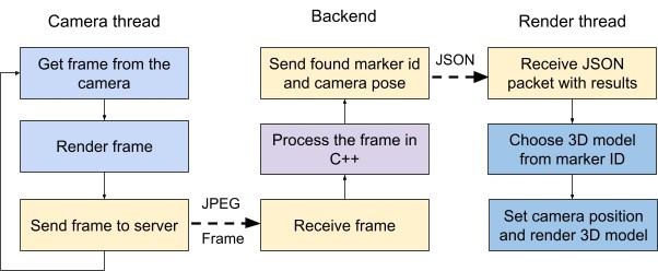
The realization with the cloud was divided into 2 separate asynchronous frontend threads and server work. Camera thread shows live-video stream from the device camera and sends jpeg to the backend. It processes a given frame and provides the id of found marker and camera pose in JSON format to the render thread. The latter one chooses a respective 3D model for found id and renders it over the real frames by Three.JS lib. The high-level logic of this pipeline is presented in Fig. 1. 

Fig.1. Server-based architecture

As a server, we used Amazon Web Services (AWS) instances. The computational power of a standard general-purpose server is enough to do the processing faster than in real-time.

However, bad quality or stability of the internet connection along with the huge distance between a user and a server lead to severe network latency and delays between threads on the front end. 

Serverless Architecture for AR

To avoid dependence on internet connection and potential lags, we introduced a front-end-only solution with the whole WebAR pipeline running on the user device. While the primary logic of the previous architecture remained unchanged, in a serverless scenario a user now has to download all files before starting the application. 

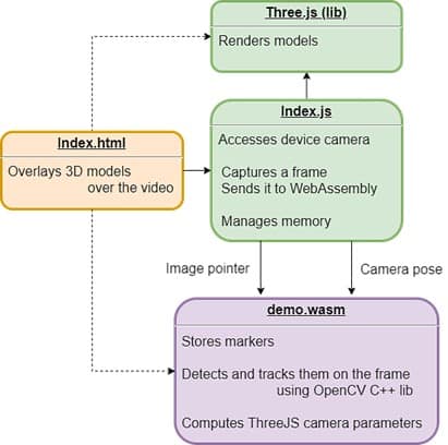
We modified and recompiled the C++ code to the WebAssembly binary code using Emscripten SDK to run it directly in the browser. This SDK is a suitable tool to call C++ functions from the JavaScript side and, additionally, speeds up the procedures. When moving to the device, we had to accelerate computer vision algorithms extensively as they are time-consuming and due to the security limitations of the web technologies. We managed to optimize them and build a real-time robust AR engine. 

Fig.2. Serverless architecture

Let’s sum up the advantages and drawbacks of each architecture:

Server-based architecture Serverless architecture
+ +
1. Provides better performance and allows to run heavy algorithms

2. Supports weak devices

1. Requires a reliable connection

2. Costly in multiuser usage scenarios

3. Network latency

1. Works without network after loading

2. Cheaper for business tasks

3. No network lags

1. Requires optimization of algorithms

Summary

Both server-based and serverless architectures are suitable for specific computer vision tasks. The server is an indispensable part of non-real-time applications that require huge computing power, e.g. CNN for object recognition or segmentation. On the other hand, pure frontend is a ‘must-have’ architecture for real-time applications.

Got interested? Check our research paper on AR in Web for more information.

Automatic Floor Segmentation Using Computer Vision

Automatic floor segmentation can serve many interesting purposes including mixed reality (MR) applications, interior design, entertainment, computation of available space in a room, or indoor robot navigation. In this project, we have been solving a problem of scene understanding and, in particular, determining which pixels of the image belong to the floor.  

The problem of floor segmentation is a good example of how the same task can be solved with classical computer vision algorithms or deep learning. As it often happens, the combination of these methods gives the best result.  

Floor Segmentation Using Classical Pipeline

We start our experiments with superpixels as they are one of the most widely adopted techniques for indoor image segmentation. We use the simple linear iterative clustering (SLIC) that works by clustering pixels based on their color similarity and proximity in the image plane. 

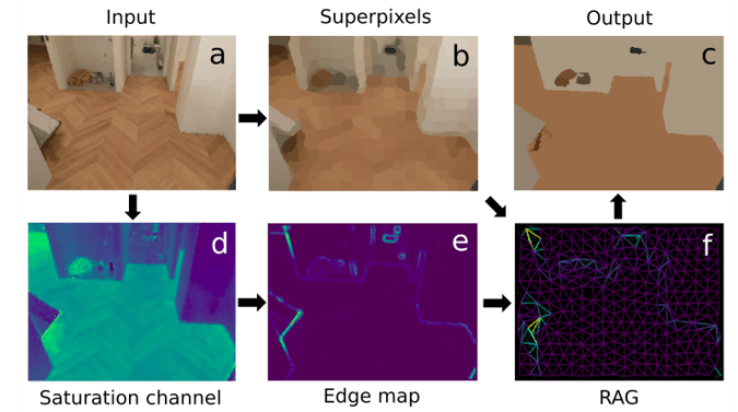
Since the straightforward application of superpixels does not provide a perfectly segmented floor, we make a more complex pipeline for image processing. Its steps are illustrated in the figure below and include:

  • transforming the RGB input image (a) into HSV color space
  • extraction of SLIC superpixels (b)
  • obtaining an edge map (e) from the S-channel image (d)
  • constructing a region of adjacency graph (RAG) (f) from the combination of the superpixels image and the edge map.
  • hierarchical merging of the RAG and final image clusterization (c)

The main steps of the classical pipeline.

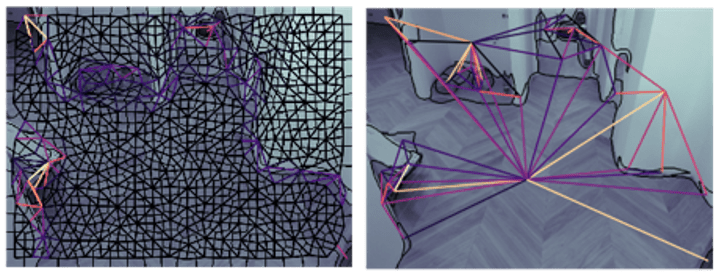
The most important step in the classical pipeline is an agglomerative hierarchical merging of the RAG. We analyze edge map intensity between each pair of neighboring superpixels and join those with edge intensity below a certain threshold. We do it iteratively starting from the weakest edges and end up with a few homogeneous regions separated by strong edges. In the figure below you can see the RAG before and after hierarchical merging. All nodes with an edge intensity less than a threshold are merged together. The border of regions is shown in black.

The RAG before (left) and after (right) hierarchical merging.

Since the classical approach is very sensitive to parameter tuning, we have run the classical pipeline several times with different model parameters, resulting in many binary segmentation masks. These masks are joined into a single one by per-pixel majority voting and additional thresholding for balancing precision and recall for a floor class.

Floor Segmentation Using Deep Learning Pipeline

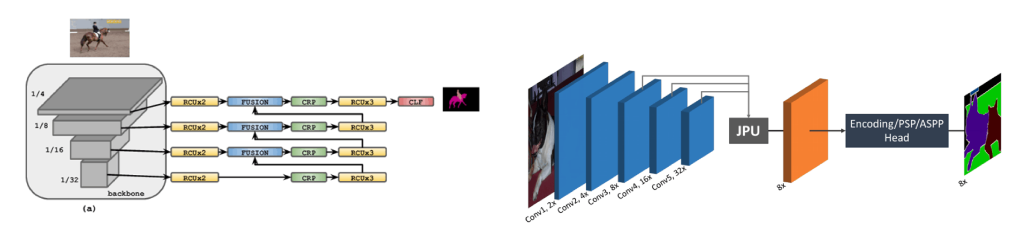
The DL solution is based on two CNNs: light-weight RefineNet and FastFCN with a joint pyramid upsampling (JPU) module and modified output layers to predict only 2 classes, a floor and not a floor.

The CNNs architectures used in the paper

For CNN training, we experimented with a few train sets: 1449 images from NYUDv2; 10329 images from the SUN-RGB-D and 8880 images from the SUN-RGB-D with NYUD removed. The target test dataset was a set of 21 hand-labeled images acquired for evaluation purposes.

Fusion of the Approaches

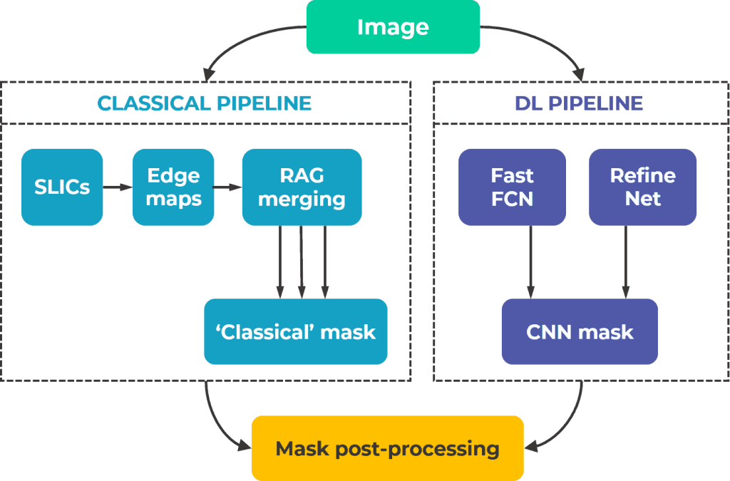
To additionally refine the quality of segmentation maps, we build a fusion scheme:

Scheme of classical and DL pipeline fusion.

The binary output mask from the classical branch is combined with the sum of segmentation masks predicted by CNNs, followed by post-processing using texture analysis. 

Post-Processing: Texture Feature Analysis and Edge Refinement

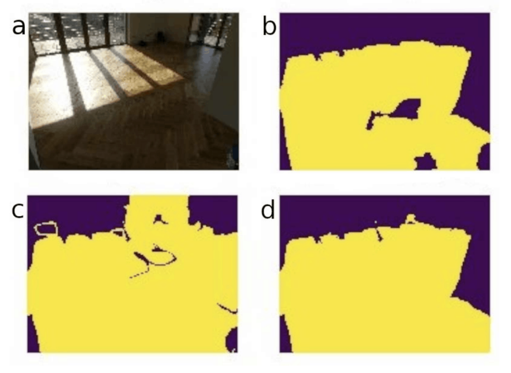
The main purpose of this stage is the final classification of uncertain areas or blobs that result from masks having opposite labels after their summation. Feature analysis resolves these uncertainties and makes a more accurate prediction. In the image below one can see an example with the input image (a), the classical pipeline output (b) the deep learning pipeline output (c) and the resulting mask after post-processing (d).

Post-processing based on the texture feature analysis. 

For texture features extraction we use a gray-level co-occurrence matrix (GLCM). It determines how often different pairs of pixels appear within a selected region (blob).

Comparison of Floor Segmentation Results

To evaluate the results of segmentation we use Intersection over Union (IoU). All intermediate IoU values are shown in the table below.

Mask obtained with: IoU
Classical branch 0.5442
RefineNet 0.7837
FastFCN 0.7893
Deep learning branch 0.7939
Classical + deep learning branches 0.7977
Full pipeline 0.8013


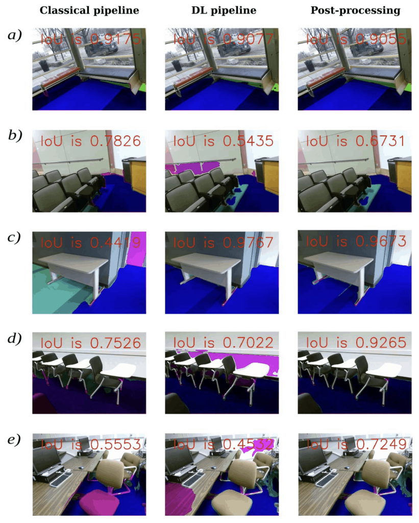
In the following figure, you can find the examples of segmentation masks obtained with the classical pipeline, deep learning pipeline, and as a result of their combination and post-processing.

 Color legend: dark blue is a  true positive, magenta is a false positive, cyan is a false negative.

The deep learning solution handles more challenging cases better than the classical computer vision pipeline. However, for some images, the developed image analysis procedure provides quite competitive results or even outperforms the CNN-based solution. The best result is achieved by merging 3 masks (two from the neural networks and one summed mask from the classical pipeline) and applying the post-processing based on texture feature analysis.

Summary

We have examined the problem of automatic floor segmentation. Despite tremendous progress in CNNs, classical CV still does a great job in pre-processing and post-processing stages as well as covers some specific classes where the pre-trained DL model might fail.

The Ultimate Guide to Developing Skills as a Computer Vision Engineer

If you want to dig into Computer Vision (CV) but have no idea where to start, this beginner guide is for you. Here we recommend some sources which will come in handy for learning and understanding both the computer vision and deep learning basics. 

When you search for a position of computer vision engineer, you’re likely to see that companies are looking for a candidate with:

  • digital image processing understanding and knowledge of classical computer vision algorithms,
  • background in mathematics,
  • sufficient skills in programming (Python and C++ are the most required),
  • knowledge of main libraries for classical CV (like OpenCV and Numpy for Python),
  • machine learning / deep learning (ML/DL) understanding,
  • knowledge of main ML/DL libraries (like TensorFlow, Keras, PyTorch)
  • experience.

Let’s now go step by step and see how and where to cover each item from the list above:

Digital Image Theory and Processing Methods

Do you know what a digital image is? How the color pixels are formed?  Have you heard about color spaces, histograms, image filters, and convolution? The video course on digital image processing presented by Prof. Guillermo Sapiro (Duke University) will be a good starting point if you answered ‘No’ to those questions. You can also check the Digital Image Processing tutorial, which is pretty simple but covers a lot. As for the books on the topic, one of the best ones is “Digital Image Processing” by Rafael Gonzalez and Richard Woods. Another book by Ian Young et al. explains the fundamentals of digital image processing and is freely available.  As for classical computer vision algorithms, Richard Szeliski’s book “Computer Vision: Algorithms and Applications” is quite comprehensive and has its free draft version available online. Want to dive into the geometry of image formation, projective transformations, or multi-view geometry? Try the course by the University of Pennsylvania on Coursera or “Multiple view geometry” book by Richard Hartley.A hint: Often tutorials on digital image processing use OpenCV examples to gain practical knowledge, so learning this topic might be useful along with exploration of the OpenCV itself (see our recommendations in #4).

Do I Need to Know Maths for Computer Vision?

When it comes to Maths, you will need linear algebra, calculus, and probability theory. Most likely, you studied them at the university. The good news is that it should be enough. Yet, refreshing the knowledge is always a good idea: an Immersive Math interactive book and video explanations of basic math concepts can help you with this. A nice overview of possible mathematical areas that can be of use for CV is given here. You can always refer to that material if you need a cheat sheet.

What Programming Language Is Needed for Computer Vision?

If you use C++, keep going, but Python is the most requested programming language in CV/ML/DL . It is easy-to-learn, powerful, and great for CV, ML, and DL tasks. Learn everything from the ground up or level-up your skills with Real Python. There are plenty of free tutorials, structured links to useful resources, and video courses available. An extensive online tutorial from Python developers is another great option to master this skill.

The knowledge of the Numpy library basics is a must-have among your skills. It is used for numerical data preparation and processing. There is a short example-based tutorial to start with. If you prefer video tutorials, check Learn NUMPY in 5 minutes.

OpenCV Is a Must

Make this open-source computer vision and machine learning software library your best friend. There are plenty of tutorials, you can start with this post to dig in, for example. A comprehensive guide on most of the functions is available as an OpenCV tutorial webpage where you can go on learning digital image processing with examples. You can always check the Learn OpenCV blog for some implemented projects.

Machine Learning and Deep Learning Libraries

Learning ML/DL libraries is useless without theory knowledge. We suggest you start by trying to understand the theory behind the ML algorithms and neural networks first and then implement it with code. Here, it would be a mistake not to mention the classics: Machine Learning course by Andrew Ng on Coursera, The Deep Learning book by Ian Goodfellow.  An online book on Neural Networks and Deep Learning by Michael Nielsen may help you, too. Just a kind warning: these are not for kids, maths formulas inside! Stanford University is also offering a couple of extensive lecture series online: Computer Vision (with deep learning) and Convolutional Neural Networks for Visual Recognition. Last, but not least, a recent course from New York University by Yann LeCunn overviews the latest techniques in deep learning and is available both in video and text formats.

Once you have mastered the basics of neural networks and their main parameters to use, it’s time to do some coding. There are two main ways to follow here: using TensorFlow [with Keras inside] from Google or PyTorch from Facebook. Knowing both of them would give you a couple of extra points, of course. Both PyTorch and Tensorflow websites offer quite comprehensive tutorials. To dive into TensorFlow even deeper, try the Hands-On Machine Learning book by Aurélien Géron. An awesome blog PyImageSearch by Adrian Rosebrock can help you a lot. Oldie but goodie AI Shack also counts. Finally, a technical blog of SicaraAI will give you examples of real CV projects.

Find a Trainee Program in Computer Vision

Now it’s time for practice! If you want to benefit the most, try searching for an internship position or a trainee program. In any case, there are a lot of examples and test datasets on the net, basically on websites from the previous item. You can always enter the competition on Kaggle, collaborate with other engineers to solve real-life problems and get a chance to practice before being employed in the real-world. Try to implement some solutions to have your pet-projects to show on job interviews and jump on board, apply for a position in a CV/ML/DL company!

Well, what else?… Let’s cover some useful tools that can ease your study:

  • Jupyter and Google Colab

When learning online you can meet the examples or tasks in Jupyter notebooks (wiki) and its online Google colab version. Practically coding there is a bit different from what is usually done in IDE. Knowing the concept of such notebooks could be helpful.

  • Git / GitHub / Bitbucket or other version control system

Git now is a standard of a version control system, which is useful not only for professional programmers but helps a lot to download examples from the net, share your projects with others, and demonstrate your experience on job interviews. You should learn the basic terminal commands and understand what’s going on. Modern IDEs usually implement Git commands in their GUI and take care of the routine tasks. 

  • Integrated development environment (IDE)

We recommend the PyCharm free community version. It is ok to use simple text editors at first, but you will need more options further. It seems more reasonable to start using IDE and learning its options step by step than switching to IDE when you suddenly realize that your favorite text editor slows down your work.

Conclusion

It’s 2021.  AI keeps pushing boundaries and entering new and new areas. The demand for computer vision/deep learning engineers is very likely to keep increasing. Get prepared for this future today 😉

iPhone’s 12 PRO LiDAR: How to Get and Interpret Data

Apple events always amaze the entire world and 2020 was not the exception. Apple presented the first mobile devices equipped with LiDAR: iPad Pro 11 and iPhone 12 Pro (and PRO max version). This active sensor measures physical distances to the objects on a spatial two-dimensional grid. Nowadays it is widespread in the automotive area for object detection and collision avoidance.

How can developers and computer vision engineers use LiDAR in their work? With a lack of technical documentation, there is no other way to answer that question except for making own experiments. In this post, we are going to show you how to create a logger to retrieve data from the iPhone’s LiDAR and an experiment on the accuracy of distance measurements with this scanner. If you want to follow our steps, you’re going to need an iPhone 12 PRO LiDAR, a ruler, a tape measure, and some spare time.

Source: https://www.forbes.com/


iOS Logger Application

First things first. In order to play with the LiDAR data, we need to store it somehow. For this purpose, we created a basic logger application that saves RGB camera frames and depth maps obtained from the scanner.

Screenshot of Logger Application

To use a logger, you need to follow four main steps:

  1. Configuring and starting ARSession,
  2. Capturing RGB and depth frames,
  3. Getting distances to the objects,
  4. Saving the results.

Let’s have a closer look at each of them. 

Step 1: Configure and Start ARSession

The logger is based on ARSession. It combines data from cameras and motion-sensing hardware to fill an ARFrame object. The latter contains all the necessary information.

Sensor data storage principle

First of all, we import the ARkit framework into our project. Then we create the ARSession and set up its configuration. This configuration consists of a set of options to enable or disable sensors or tell ARKit how to process given data for a better user experience. As default settings, we choose ARWorldTrackingConfiguration, which tracks changes in translation and rotation of the device (6 Degrees of Freedom).

import UIKit
import ARKit
import Zip

class ViewController: UIViewController, ARSessionDelegate{
    var session: ARSession!
 
    override func viewDidLoad() {
        super.viewDidLoad()

        session = ARSession()
        session.delegate = self
    }
    
    override func viewWillAppear(_ animated: Bool) {
        super.viewDidAppear(animated)

        let configuration = setupARConfiguration()
        session.run(configuration)
    }  

    func setupARConfiguration() -&amp;amp;gt; ARConfiguration{
        let configuration = ARWorldTrackingConfiguration()

	  // add specific configurations
	  ...
	  return configuration
    	}
}

Since we want to get depth data from LiDAR, we need to check whether our device supports this sensor and enable its flag ‘.sceneDepth’ in ARConfiguration.


func setupARConfiguration() -&gt; ARConfiguration{
    let configuration = ARWorldTrackingConfiguration()

    // add specific configurations
    if ARWorldTrackingConfiguration.supportsFrameSemantics(.sceneDepth) {
        configuration.frameSemantics = .sceneDepth
    } 

    return configuration
}

ARSession is ready.

Step 2: Capture RGB and Depth Frames

The next step is to capture ARFrame at the specific moment. For this purpose, we added UIButton “SaveFrame” on the display. By clicking on it, you receive the current ARFrame with full information from enabled sensors from ARSession. 

@IBAction func onSaveFrameClicked(_ sender: Any) {
    	if let currentFrame = session.currentFrame {
        	let frameImage = currentFrame.capturedImage
        	let depthData = currentFrame.sceneDepth?.depthMap

	      // Process obtained data
            ...
      }
}

This code loads the RGB frame and depth map as ‘CVPixelBuffer’ objects. Additionally, ‘sceneDepth’ contains a confidence map. You might want to take a closer look at it since depth data can be incorrect in the case of surfaces with varying reflectivity. 

Let’s now move to prepare the RGB frame and depth map for saving. For that, we convert pixel buffers into ‘UIImages’ in almost the same way. As depth is supported by the limited number of devices, it is an optional type.

if let currentFrame = session.currentFrame {
       ...
      // Process obtained data
      // Prepare RGB image to save
      let imageSize = CGSize(width: CVPixelBufferGetWidth(frameImage),
                            height: CVPixelBufferGetHeight(frameImage))
      let ciImage = CIImage(cvPixelBuffer: frameImage)
      let context = CIContext.init(options: nil)
        	
      guard let cgImageRef = context.createCGImage(ciImage, from: CGRect(x: 0, y: 0, width: imageSize.width, height: imageSize.height)) else { return }
      let uiImage = UIImage(cgImage: cgImageRef)

      // Prepare normalized grayscale image with DepthMap
      if let depth = depthData{
           let depthWidth = CVPixelBufferGetWidth(depth)
           let depthHeight = CVPixelBufferGetHeight(depth)
           let depthSize = CGSize(width: depthWidth, height: depthHeight)
		
	     ...

           let ciImage = CIImage(cvPixelBuffer: depth)
           let context = CIContext.init(options: nil)
           guard let cgImageRef = context.createCGImage(ciImage, from: CGRect(x: 0, y: 0, width: depthSize.width, height: depthSize.height)) else { return }
           let uiImage = UIImage(cgImage: cgImageRef)
}

While the size of the RGB frame is 1920×1440, the depth map is quite small, only 192×256.

However, even a small resolution of a lidar depth map could be very helpful in object detection or background subtraction tasks.

Step 3: Distances to the Object

Depth UIImage is a normalized grayscale image. Distances are encoded in brightness, the closest objects are dark, while the further ones are light. 

While for some tasks it is enough to have relative distances, we need to get the real physical values in our case. To get LiDAR distances in meters, we need to read CVPixelBuffer as Float32. In the code below, we fill a 2-dimensional array ‘distancesLine’ with raw depth data.


if let depth = depthData{
    let depthWidth = CVPixelBufferGetWidth(depth)
    let depthHeight = CVPixelBufferGetHeight(depth)
    CVPixelBufferLockBaseAddress(depth, CVPixelBufferLockFlags(rawValue: 0))
    let floatBuffer = unsafeBitCast(CVPixelBufferGetBaseAddress(depth),
				 		to: UnsafeMutablePointer&amp;amp;lt;Float32&amp;amp;gt;.self)
           	 
    for y in 0...depthHeight-1{
        var distancesLine = [Float32]()
        for x in 0...depthWidth-1{
            var distanceAtXYPoint = floatBuffer[y * depthWidth + x]
            distancesLine.append(distanceAtXYPoint)
            print(&quot;Depth in (\(x),\(y)): \(distanceAtXYPoint)&quot;)
        }
        depthArray.append(distancesLine)
    }     	
		...

Depth data spans from floatBuffer[0] up to [height * width]. In our case, there are 192 rows and 256 columns, 49152 elements in total. Keep in mind that floatBuffer is just a pointer to the memory address with depth information. Like in C++, the pointer does not know anything about the real size of the depth array, so you can easily go out of the limits without any warning. 

Step 4: Save Results

Finally, we need to save our results to the device folder to have an opportunity to analyze them. The following auxiliary code creates a folder, gets its path, and clears the folder in case it was built before.


func getTempFolder() throws -&amp;amp;gt; URL {
    let path = try FileManager.default.url(for: .documentDirectory, in: .userDomainMask, appropriateFor: nil, create: true
).appendingPathComponent(&quot;tmp&quot;, isDirectory: true)
        
    if (!FileManager.default.fileExists(atPath: path.path)) {
       do {
           try FileManager.default.createDirectory(atPath: path.path, withIntermediateDirectories: true, attributes: nil)
       } catch {
               print(error.localizedDescription);
       }
    }
    return path
}


func clearTempFolder() {
    let fileManager = FileManager.default
    let tempFolderPath = try! getTempFolder().path
    do {
        let filePaths = try fileManager.contentsOfDirectory(atPath: tempFolderPath)
        for filePath in filePaths {
            try fileManager.removeItem(atPath: tempFolderPath +    
                                               filePath)
        } 
    } catch {
            print(&quot;Could not clear temp folder: \(error)&quot;)
    }
}

The folder should be created when setting up our ARSession.

override func viewDidLoad() {
    	super.viewDidLoad()
   	 
    	clearTempFolder()
   	 
    	session = ARSession()
}

Now, we can save images and depth array as a .txt file. 

// Save image (the same for depth)
let imagePath = try! getTempFolder().appendingPathComponent(&quot;\(frames.count).jpg&quot;)
try! uiImage.jpegData(compressionQuality: 0.9)?.write(to: imagePath)


// Save depth map as txt with float numbers
var depthTxtPath=try! getTempFolder().appendingPathComponent(&quot;\(frames.count)_depth.txt&quot;)
let depthString:String = getStringFrom2DimArray(array: depthArray, height: depthHeight, width: depthWidth)
try! depthString.write(to: pathTxt, atomically: false, encoding: .utf8)


// Auxiliary function to make String from depth map array
func getStringFrom2DimArray(array: [[Float32]], height: Int, width: Int)-&gt;String{
    var arrayStr: String = &quot;&quot;
    for y in 1...height-1{
   	 var lineStr = &quot;&quot;
   	 for x in 1...width-1{
   		 lineStr += String(array[y][x])
   		 if x != width-1{
   			 lineStr += &quot;,&quot;
   		 }
   	 }
   	 lineStr += &quot;\n&quot;
   	 arrayStr += lineStr
    }
    return arrayStr
}

LiDAR Experiments

Now we are ready to compare the measured depth by LiDAR with real physical distances to objects. ARKit documentation suggests avoiding highly reflective or light-absorbing surfaces. The company’s poster meets these requirements perfectly, so we used it as a target.  We fixed a smartphone with a tripod and centered the object on the screen. 

Scene configuration

As long as we were dealing with a flat and distributed object, it was enough to take the data just from the central pixel of the depth map. We recorded the LiDAR data for distances from 20 cm up to 5.5 m. We used a 5 cm measurement step for distances up to 1 m and a 50 cm step for the larger ones. The distance was captured by LiDAR a few times to evaluate the repeatability of the results. Here is what we obtained.

Experimental results

One can see that LiDAR provides reasonable accuracy for distances of up to 4 meters which is sufficient for portrait mode and short-range AR. The higher distances provided different results for every button click (see error bars in the figure above). This indicates the limits for the iPhone’s LiDAR operation range. 

Summary

Definitely, the iPhone Lidar sensor is interesting to play with. We hope that provided code snippets and findings will be useful for those who are willing to examine the new LiDAR sensors. Our iPhone experiments are definitely to be continued. Stay tuned!