JAX: Can It Beat PyTorch and TensorFlow?

Historically, there have been many Deep Learning (DL) frameworks, like Theano, CNTK, Caffe2, and MXNet. Nowadays, they appear to be dead or dying, as just two frameworks heavily dominate the DL scene: Google TensorFlow (TF), which includes Keras; and PyTorch from Meta aka FaceBook. However, there is no reason to believe such a duopoly will persist forever. All the time, new DL frameworks are proposed. We have no idea which DL framework will be popular in, say, ten years.

One of the more serious contenders in the ”DL framework Junior League” is Google JAX. In this article, we examine JAX and look at its positive and negative sides. We will address questions like “When to use JAX?” and “Does JAX have any chance of success?”. But first, why was JAX created? We don’t know exactly, but apparently, AI folk in Google got fed up with TensorFlow and wanted a new toy to fool around with.

To understand JAX, note that Google has not one, but at least two (perhaps more) competing AI teams: Google Brain and DeepMind. They seem to never agree on anything. Even in the TensorFlow era, DeepMind used their own layer API called Sonnet (instead of the usual Keras). Probably nobody outside of DeepMind has ever heard of it. Now history repeats itself with JAX. 

JAX ecosystem consists of the following packages (which are separate PIP packages):

  • JAX: Low-level API (like torch without torch.nn or TF without tf.keras)
  • FLAX (FLexible JAX): Layer API from Google (excluding DeepMind)
  • Haiku: Another layer API, from DeepMind, inspired by Sonnet (TF)
  • OPTAX: Optimizers and loss function for JAX
  • Numerous more specialized packages: Trax, Objax, Stax, Elegy, RLax, Coax, Chex, Jraph, Oryx … . See the JAX ecosystem article.

Note that currently, JAX has no dataset/dataloader API, nor standard datasets like MNIST. Thus you will have to use either TF or PyTorch for these tasks or implement everything yourself.

JAX is open-source, it has pretty good documentation and tutorials. We also recommend AI Epiphany lectures on JAX and Flax. We assume that the reader has basic DL and python knowledge and some experience with either TF or PyTorch.

JAX: Basics, Pytrees, Random Numbers & Neural Networks

JAX Basics and Functional Programming

JAX (the low-level API) has two predecessors:

  • autograd: Numpy-like library with gradients (backprop)
  • Google XLA (accelerated linear algebra): fast matrix operations for CPU, Nvidia GPU and TPU. It compiles stuff into an efficient machine code. It is optional in TensorFlow, but required by JAX.

You can view JAX as “numpy with backprop, XLA JIT, and GPU+TPU support”. You write code like in numpy, but use the prefix jnp. (jax.numpy.) instead of np. . Then your code can run on CPU, GPU, or TPU with no changes. At least, this is the theory. Practice can be a bit harder. GPU installation requires precise versions of CUDA and CUDNN, just like for TensorFlow. It is only practical in Docker. However, unlike TF, JAX has no official docker images yet. And unless you work for Google, you will probably never see a TPU anywhere outside Google Colab.

Apart from the numpy-like API, JAX includes the following main operations:

  • Calculate gradients with jax.grad()
  • Compile python code to XLA with jax.jit()
  • Add batch dimension to a function using jax.vmap() or jax.pmap()

The biggest difference between numpy and JAX is that JAX is heavily into functional programming; thus, JAX arrays (aka tensors) are always immutable. What does “functional programming” mean? It means that the python functions must be “pure”, e.g., behave like mathematical functions. In particular, a function f(x, y, z) is PURE if:

  • It receives input data ONLY through the arguments x, y, z
  • It outputs results ONLY through the return value(s)
  • It does NOT modify objects x, y, z
  • It does NOT access any global variables
  • It does not print anything, does not access the screen, keyboard, any files or devices, or OS API

The function which breaks these rules is not pure, and we say that it has “side effects”. Such functions are not allowed in functional programming.

But what about classes and objects? The vanilla functional programming does not allow any classes. However, it would be highly impractical in Python, where we need classes for objects like multidimensional arrays. Thus JAX makes a compromise: classes and objects are allowed as long as they are strictly immutable: created once and never changed. What does it mean for DeepLearning? It means that any DL object, such as a model (neural net) or optimizer, must be separated into the immutable object (containing the code) and mutable parameters and state. In particular, the following data objects (usually python dictionaries) are separated from the main immutable objects (containing the code):

  • Neural network parameters (which are trained)
  • Neural network state (which is not trained, e.g., BatchNorm state)
  • Optimizer state
  • Random number generator (RNG) state.

Note that all this is very different from e.g. PyTorch, where a model, optimizer and RNG are all mutable objects under the hood, containing their own states and parameters. Moreover, the RNG is global. Functional programming in JAX makes things clearer for an experienced DL engineer, as you don’t have to worry about many ways the objects can be modified. All modifications are always explicit! On the other hand, it can make JAX harder to understand for beginners compared to PyTorch or TF.

How do you work with the immutable JAX arrays? A typical numpy code

a = np.arange(5.)

a[1:3] = [-1., -2.]

will not work in JAX, as the array a is modified in-place. Instead, you will have to write the following:

a = jnp.arange(5.)

a = a.at[1:3].set([-1., -2.])

Here, the object a is not modified but replaced by a new python object.

jax.jit(): Make a Python Function Run Much Faster

Suppose you have a python function my_function. According to JAX tutorials, you can make a python function faster by JIT-compilig it with jax.jit(). Actually, it’s compiling with XLA. Sounds too good to be true? It is.

Of course, magically accelerating any arbitrary python function will be impossible (unless you port it to C++). What’s the catch? Let’s see how exactly jax.jit() works. What happens when you type

fast_function = jax.jit(my_function)

?

  • my_function is compiled from python to XLA. It’s achieved by tracing, similar to torchscript tracing in PyTorch. Actually, to be precise, the tracing happens when fast_function is called for the first time.
  • Tracing takes significant time, so such “optimization” only makes sense if we are going to call fast_function repeatedly many times without recompiling.
  • XLA is optimized to particular types of input arguments and particular shapes and dtypes of input jnp arrays. If input shape or type changes, fast_function is automatically recompiled, which takes time.
  • Python statements such as if and for are not allowed unless they involve only arguments declared static. If the value of a static argument changes, the function is recompiled.
  • Function my_function is supposed to be pure. In reality, if a side effect like print() is present, it works at the tracing stage, but NOT when running fast_function without recompiling.

Despite all these limitations, JIT can accelerate JAX code significantly when used correctly and is routinely used in most JAX codes.

Note that jax.jit() is often used as a decorator:

@jax.jit
def my_function(x):

    …

jax.grad() : Gradients of a Scalar Function

Probably the most important JAX function is jax.grad(), which implements the gradients (backprop), which are a must for neural network training. Minimal example:

def f(x):

         return jnp.sum(x ** 2)

gf = jax.grad(f)

x = jnp.array([1., 2., 3.])

print(f(x), gf(x)) # Prints 14.0 [2. 4. 6.]

Function f() must return a scalar. If it has multiple arguments, jax.grad() differentiates with respect to the first one. jax.grad() also uses tracing, but now if and for statements are allowed. A useful variation called jax.value_and_grad(f) creates a function which returns a tuple (f(x), grad(f)(x)).

jax.vmap() and jax.pmap(): Vectorize a Function along the Batch Dimension

Sometimes you have a function that works on, say, a vector, but you want to make it accept batches (one extra dimension). For example, let’s define a function:

def f(x):                     

         w = jnp.array([[0., 0., 1.], [0., 1., 0.], [1., 0., 0.]])

         return jnp.dot(w, x)

It works on the shape (3,) only, but not (B, 3), where B is the batch size. You can then transform function f with jax.vmap() to make it batch-compatible:

vf = jax.vmap(f)         # Add a batch dimension to function

x = jnp.array([[1., 2., 3.], [4., 5., 6.]])   # shape (2, 3)

print(f(x))          # Error  ! Wrong shape of x !

print(vf(x))        #  Success :  [[3., 2., 1.], [6., 5,. 4.]]

Note: this function is similar to the numpy-derived function jnp.vectorize(), but the two differ in details.

There is a parallel version called jax.pmap(), which distributes the computation across multiple XLA devices (GPUs, TPUs or CPU cores). Note that while CPU cores are separate devices, GPU cores are not. There is also a rudimentary API for inter-thread communication: psum(), pmean(), pmax(). Unfortunately, jax.pmap() strictly requires that the batch size B must be smaller or equal to the number of XLA devices. It is too stupid to distribute the threads otherwise! Note that if you are running on a CPU, by default JAX uses only one CPU core. To force JAX to use 8 CPU cores, write:
os.environ[‘XLA_FLAGS’] = ‘–xla_force_host_platform_device_count=8’

To check the available devices, write:
print(‘n_devices=’, jax.local_device_count())

print(‘devices=’, jax.devices())

JAX Pytrees

As we mentioned, various parameters and states must be kept separate from the immutable model objects. They are typically kept in a nested structure of python dict() and list() or similar classes. Such objects are called pytrees in JAX. Their leaves (lowest-level nodes) are typically JAX arrays. 

Functions like jax.grad() support pytrees. For example, if the first argument p of a function f(p, x) is a pytree, the gradient with respect to p means a pytree of the same structure as p, consisting of gradients with respect to each leaf in p. This is a routine for neural nets; if f(p, x) is a JAX model, then the first argument p is typically a pytree of the network parameters (which we train).

There are a couple of useful functions to work with pytrees. jax.tree_map() applies a unary function to each node in a pytree, generating a new pytree of the same structure. For example, to print the pytree of the shapes of all parameters in the pytree t, type:

print(jax.tree_map(lambda x: x.shape, t))

A similar function jax.tree_multimap() applies a binary operation to two pytrees of the same structure. For example, the “sum of two trees t1 and t2” is given by:

jax.tree_multimap(lambda x, y: x+y, t1, t2)

JAX Random Numbers

Random numbers in JAX can confuse people who are used to numpy or PyTorch. Because of the functional programming paradigm, stateful or global random number generators (RNGs) are not allowed in JAX. How do you implement an RNG without a mutable state? Here we see the first example of how code and state are separated in JAX. Essentially the same logic applies to other objects like models and optimizers.

The function jax.random.normal() requires a “key”, which is the RNG state. You can create the key from a random seed like this (RNG initialization):

key = jax.random.PRNGKey(2022)

Then you can create a random array like this:

print(jax.random.normal(key, (2,)))

Everything works, right? Not really! If you put the same statement again, you will get exactly the same result:

print(jax.random.normal(key, (2,)))

This is the blessing and the curse of functional programming. Everything is explicit, predictable, clear, and immutable. In this case, the same state key results in the same random array. 

How to generate random numbers properly? For that you need a function jax.random.split(), which generates two (or more) keys from the input key. Each key must be used only once (strictly !). Every time you need a random number, you write the following code:

key1, key = jax.random.split(key)            # Split key1, update key
print(jax.random.normal(key1, (2,)))          # Use key1 only once !

Don’t forget to split a new key (key1) every time you generate a new random number, because you can use each key only once! Alternatively, you can split multiple keys at once:

key1, key2, key3, key = jax.random.split(key, 4)   # Generate 3 keys, update key

or even a list of keys:

*keys, key = jax.random.split(key, 10 + 1)   # Generate a list of 10 keys, update key

One more thing: if a neural net requires an RNG for inference (e.g., it has dropout), the RNG key must be supplied explicitly at the inference time. You will see examples of this below.

Side note: of course, nothing stops you from using the numpy RGN and converting the result to JAX, but it is considered a bad style among JAX developers.

A Minimal Neural Net in Pure JAX

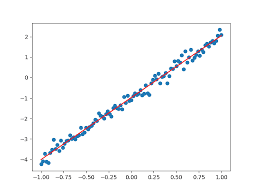
Let’s use our knowledge to code a trivial neural net in pure JAX. We want to implement a linear regression. Let’s create our data, a linear function plus some random noise:

n = 101

xx = jnp.linspace(-1, 1, n)

key_noise, key = jax.random.split(key)

yy = 3 * xx – 1 + 0.2 * jax.random.normal(key_noise, (n,))

Now we create a linear model with two parameters:

def model(params, x):

         return params[0] * x + params[1]

Note how the first argument (which we usually take a gradient over) is a pytree of the optimizable network parameters (just a size-2 list in this case).

Next, we define a loss function, compile it with jax.jit(), and calculate its gradient (with respect to params):

@jax.jit

def loss_fun(params, x, y):

         pred = model(params, x)

         return jnp.mean((y – pred) ** 2)

vgl = jax.value_and_grad(loss_fun)

Finally, we initialize the parameters and perform the training loop:

params = [1., 1.]

lr = 0.1

for i in range(100):

         loss, grad = vgl(params, xx, yy)

         params = jax.tree_multimap(lambda p, g: p – lr*g, params, grad)

         print(i, loss)

Note how we use jax.tree_multimap() to update our parameters (the vanilla SGD optimizer). The result looks like this:

OPTAX

This is going to be the shortest chapter of this article. In the previous example, we implemented vanilla SGD using jax.tree_multimap(). But we know it is better to use more advanced optimizers like Adam or SGD+momentum. Here, OPTAX comes to the rescue. Let’s see how we can modify the previous example using OPTAX. Since this is JAX, we must create an optimizer object (immutable, code-only) and then a state for it: 

params = [1., 1.]

lr = 0.1

optimizer = optax.adam(learning_rate=lr)   # Create the optimizer

opt_state = optimizer.init(params)        # Init optimizer state

Next, we rewrite the training loop by using the optimizer:

for i in range(100):

         loss, grad = vgl(params, xx, yy)

         upd, opt_state = optimizer.update(grad, opt_state)  # Optimizer step

         params = optax.apply_updates(params, upd)       # Basically params + upd

         print(i, loss)

First, the method optimizer.update() calculates the updates plus the new optimizer state. Second, we add the updates to the params using optax.apply_updates(), which is basically just a sum of two pytrees using jax.tree_multimap() under the hood.

Note that we use the same OPTAX optimizers regardless of whether our model is written in pure JAX, FLAX, or Haiku. Apart from optimizers, OPTAX also contains several loss functions and schedulers.

FLAX

FLAX: Basics

FLAX (FLexible JAX) is a layer API for JAX created by Google (DeepMind excluded). It plays a role similar to Keras in TF or torch.nn in PyTorch. We are going to use the modern flax.linen API, typically imported as nn; the old API flax.nn is deprecated and removed!

Let’s create a FLAX model of a single linear (aka FC aka Dense) layer:

model = nn.Dense(features=3)

This creates an (immutable) model object, but we also have to create and initialize the model parameters. For that, you need two things: a single-use random key key_init, and a sample input x (to specify input shape):

x = jnp.ones((4, 2))                            #  Sample input: batch_size=4, dim=2

key_init, key = jax.random.split(key)

params = model.init(key_init, x)     

Now, let’s print the parameter shapes:

print(‘params:’, jax.tree_map(lambda p: p.shape, params))

The output looks like this:

params: FrozenDict({

         params: {

                  bias: (3,),

                  kernel: (2, 3),

         }, })

What on earth is a “FrozenDict”? Basically, it’s an immutable python dict, defined in FLAX and registered with the JAX pytree ecosystem (which allows registering custom collection types). FLAX models prefer FrozenDict, but they can take python dict as well.

If the dictionary params consist of model parameters, why does it have a subdictionary named “params”? We’ll see it in a moment.

To run a model inference (or training) on a single input x, you type:

y = model.apply(params, x)

Note that you cannot use the parentheses operator! If the model requires a random key (e.g., for dropout), you’ll have to supply it as well:
y = model.apply(params, x, rngs={‘dropout’: key_do})

FLAX Models

But how can we create a FLAX model of more than one layer? There are several options. First, we can use sequential models (since FLAX 0.4.1):
model = nn.Sequential([

         nn.Dense(features=5),

         nn.relu,

         nn.Dense(features=3),

])

Note that nn.Dense() is a FLAX model object, while nn.relu is a function (with no parameters), nn.Sequential() supports both. 

For more serious models we’ll have to inherit the nn.Module class. Note that this class is a python dataclass (read about them if you didn’t already, they are fun):

class GoblinModel(nn.Module):

         feat1: int

         feat2: int


         def setup(self):                                  # This is called when init() is called

                  self.d1 = nn.Dense(self.feat1)       # A Submodule is registered

                  self.d2 = nn.Dense(self.feat2)


         def __call__(self, x):

                  x = jax.nn.relu(self.d1(x))             # Note: no apply(), no params !

                 return self.d2(x)

A dataclass defines several strictly-typed features (feat1, feat2 in our case) and automatically creates a constructor for them. That is why we should not define an explicit constructor in a dataclass, and the method setup() is used instead. It is called when you call the init() method of the model. Now we can create a model instance as usual followed by the initialization:
model = GoblinModel(5, 3)  # (feat1, feat2)

x = jnp.ones((4, 7))               #  Sample input: batch_size=4, dim=7

key_init, key = jax.random.split(key)

params = model.init(key_init, x)

A lot of magic happens under the hood when we call init(). It calls setup() and all submodules defined in setup() are registered, i.e. they are added to the parameter dictionary and initialized. Also init() handles random number keys under the hood and automatically generates a new single-use key for initializing each layer.

Note how in the __call__() method the submodules are called directly without giving them any parameters. When we run the inference, we actually call apply() and not __call__(), and the former method handles all parameters and passes all submodule parameters to the respective submodules.

However, the syntax with setup() is  somewhat cumbersome, thus people often use the decorator nn.compact() (a lot of black magic happens in this function) to define the submodules directly in __call__():

class OrcModel(nn.Module):

         feat1: int

         feat2: int


         @nn.compact

          def __call__(self, x):

                  x = nn.Dense(self.feat1)(x) # Layer    

                  x = jax.nn.relu(x)                # Function

                  return nn.Dense(self.feat2)(x)


A CNN example (CNNs are popular in computer vision) is not much harder:

class DwarfCNN(nn.Module):

         @nn.compact

         def __call__(self, x):

                  x = nn.Conv(features=32, kernel_size=(3, 3))(x)    # Layer

                  x = nn.relu(x)                                                         # Function

                  x = nn.avg_pool(x, window_shape=(2, 2), strides=(2, 2))

                  x = nn.Conv(features=64, kernel_size=(3, 3))(x)

                  x = nn.relu(x)

                  x = nn.avg_pool(x, window_shape=(2, 2), strides=(2, 2))

                  return x

FLAX models (custom layers)

So far, we created models out of standard FLAX layers. But how do we create a custom one? Here is an example. We use the method param() to define parameters:
class ElfLinear(nn.Module):

         feat: int

         w_init: typing.Callable = nn.initializers.lecun_normal()

         b_init: typing.Callable = nn.initializers.zeros


         @nn.compact

         def __call__(self, x):

                  w = self.param(‘w’, self.w_init, (x.shape[-1], self.feat))

                  b = self.param(‘b’, self.b_init, (self.feat,))

                  return x @ w + b

Due to the nn.compact() magic, we can declare the parameters directly in __call__() using the param() method. We need to supply an initializer and the shape. The latter is (in our example) derived from the input x, the sample input provided at the initialization. 

The Problem of State

But what if our model has a state (variables that are NOT trainable parameters)? For example, BatchNorm and related ..Norm layers have a state, and so do all models containing a BatchNorm as a submodule. This is where FLAX gets a bit awkward, in our opinion. We initialize the model as usual:

vars0 = model.init(key_init, x)

However, now the FrozenDict vars0 contain not only parameters (in the section params), but also state variables in other sections. Now we have to separate the two by hand:

state, params = vars0.pop(‘params’)

It is very important that the optimizer optimizes only parameters (params) and not vars0! In other words, we use params when initializing the optimizer and performing the optimizer updates. 

Before running apply(), we recombine parameters and state back into the dictionary vars, and use the form of apply() which updates the state. If we don’t want to update the state (a frozen BatchNorm at testing stage), we use the regular apply() instead:

vars = {‘params’: params, **state}

pred, state = model.apply(vars, x, mutable=state.keys())

Once again:

  • We must separate all model variables into state and param.
  • param (Network parameters) are optimized by the optimizer (via backprop).
  • state (Network state, e.g. batchnorm state) is updated in apply() during training, but is frozen during testing.

Do you think handling all the different parameters and states is awkward? We agree. However, for common training scenarios, FLAX provides a higher-level API FLAX TrainState, which combines model, parameters, and optimizer together. You can try it if you want. This is the highest possible level DL API, like fit() in Keras, or PyTorch Lightning.

Haiku

Haiku basics

Haiku is another layer API from DeepMind. Compared to FLAX, it is even purer functional programming. In FLAX, a lot of magic was buried in the nn.Module class and nn.compact() function. In contrast, in Haiku a model class does not matter. There is a class hk.Module, but it’s a thin submodule container that does almost nothing, and you don’t have to use it at all if you don’t want to. All elven magic happens in the function hk.transform() and its variations. Let’s see how it all works.

A neural net is always defined as a function (similar to the functional definition in Keras), for example:

def forward(x):

         return hk.Linear(3)(x)

Note that you define a Haiku module hk.Linear inside the function and do not provide any initialization data like input shape or a RNG key. Such a function will not work directly! Instead, you must transform it like this.

model = hk.transform(forward)

This step is similar to creating a functional Keras model (tf.keras.Model) in TensorFlow.

Now we get a transformed model object model. It works sort of like the FLAX module, but we never create such objects explicitly, only via hk.transform(). We still have to initialize it:

params = model.init(key_init, jnp.zeros((5, 2)))

Initialization is pretty much identical to the one in FLAX.

To run the model, we call apply():

y = model.apply(params, key_apply, x)

Note that in Haiku you must supply a RNG key in apply(), whether or not your model actually needs it (e.g., has dropout layers). If you want to get rid of this key, use an extra transformation:

model = hk.without_apply_rng(hk.transform(forward))

params = model.init(key_init, jnp.zeros((5, 2)))

y = model.apply(params, x)

A special version of hk.transform() is used when your model has a state (e.g. BatchNorm state):
model = hk.transform_with_state(forward)

params, state = model.init(key_init, x)                    # Init params + state

y, state = model.apply(params, state, key_apply, x)  # Apply model, update state

Only params are optimized. Note how Haiku separates params and state automatically, while in FLAX you had to do it by hand.

Haiku models

How do you define a model in Haiku? First, you can inherit hk.Module:

class GoblinMLP(hk.Module):

         def __init__(self, name=’goblin_mlp’):

                  super(GoblinMLP, self).__init__(name=name)

                  self.l1 = hk.Linear(5)

                  self.l2 = hk.Linear(3)


         def __call__(self, x):

                  x = jax.nn.relu(self.l1(x))

                 return self.l2(x)

You’ll still have to define a forward function (or lambda):

def forward(x):

         return GoblinMLP()(x)

But it’s Haiku, so you don’t have to use the model class if you don’t want to. How about this:

def forward_goblin(x):

         x = hk.Linear(5)(x)

         x = jax.nn.relu(x)

         return hk.Linear(3)(x)

It works, you can actually register layers in the forward function, without using the hk.Module class at all!

If you are writing a custom module, use hk.get_parameter() to register network parameters:

class GoblinLinear(hk.Module):

         def __init__(self, osize, name=’goblin_linear’):

                  super(GoblinLinear, self).__init__(name=name)

                  self.osize = osize


         def __call__(self, x):

                  n_in, n_out = x.shape[-1], self.osize

                  w_init = hk.initializers.TruncatedNormal(1. / np.sqrt(n_in))

                  w = hk.get_parameter(‘w’, shape=[n_in, n_out], dtype=x.dtype, init=w_init)

                  b = hk.get_parameter(‘b’, shape=[n_out], dtype=x.dtype, init=jnp.ones)

                  return jnp.dot(x, w) + b

You can even use parameters directly in forward(), without any hk.Module.

Haiku has a couple of further nice things. You can define an MLP (multi-layer dense network) concisely (it uses ReLU by default, this can be changed):
hk.nets.MLP([20, 20, 1])

There is also a number of standard architectures (but alas no pre-trained weights for them):

hk.nets.MobileNetV1

hk.nets.ResNet18, 34, 50, 101, 152, 200

So, Can JAX Succeed?

We don’t know it. But here are the good and bad sides of JAX, in our opinion (as compared to PyTorch and TensorFlow):

The good:

  • JAX is very TPU friendly and has built-in support for multiple devices.
  • Functional programming makes things a bit cleaner (but only for pros).
  • The weight of Google behind it should matter.

The bad:

  • It is still in the 0.x versions, the API might change.
  • Functional programming can be annoying for beginners.
  • Apart from the TPU, there are few real advantages over PyTorch (or TF).
  • There are very few deploy options. Currently, there is only the experimental jax2tf converter. No ONNX, tflite or TensorRT.
  • There is no dataset/dataloader API.
  • There are still very few existing or pre-trained models (but see flaxmodels).

Have fun and enjoy JAX! And if we you are more into video content, we have a lecture on JAX on our YouTube channel:

P.S. If the author were Google, he would create some nice deployment system for JAX, like tflite, but based on XLA, with versions for C++, Android, iOS, embedded and Web browser.

GStreamer C++ Tutorial

In the previous article, we’ve learned what GStreamer is and its most common use cases. Now, it’s time to start coding in C++. This tutorial does not replace but rather complements the official GStreamer tutorials. Here we focus on using appsrc and appsink for custom video (or audio) processing in the C++ code. In such situations, GStreamer is used mainly for encoding and decoding of various audio and video formats.

GStreamer C++ Basics

GStreamer C++ API is introduced rather well in the official tutorial, I’ll give only a very brief introduction before focusing on appsrc and appsink, the most important topic of interest to us. Our tutorial can be found here. In our code, we use C++, not C. Also, unlike the official tutorial, we are not too eager to use GLib functions like g_print().

Let’s get going. Our first example, fun1, is an (almost) minimal C++ GStreamer example. Before doing anything with GStreamer, we have to initialize it:

gst_init(&argc, &argv);

It loads the whole infrastructure like plugin registry and such. But why does it need pointers to argc, argv? You can put nullptr, nullptr if you really want to. But honestly providing your command line arguments allows gst_init() to parse GStreamer-specific flags. For example, I always add –gst-debug-level=2 to the command line in order to log warnings and errors to the console (there’s no logging by default). Interestingly, GStreamer removes all its flags from argc, argv, so that you can later parse the remaining arguments.

Next, we create a pipeline from a string

string pipelineStr = “videotestsrc pattern=0 ! videoconvert ! autovideosink”;

GError *err = nullptr;

GstElement *pipeline = gst_parse_launch(pipelineStr.c_str(), &err);

checkErr(err);

MY_ASSERT(pipeline);

Where MY_ASSERT is my assertion macro (like CV_ASSERT, never ever use the C++ assert statement !), and checkErr is my function that checks a GError object for errors, see the code for details. Checking for errors is important, to catch any typos in the pipeline string, linking failures etc. GStreamer is heavily based on GLib, especially on the GObject framework (a part of GLib), a pure C object-oriented framework. All GStreamer entities are GObject objects and they are handled as raw pointers. This may seem ugly compared to modern C++, but there is nothing I can do about it (as gstreamermm is now dead).

Now we created the pipeline, we should play it

MY_ASSERT(gst_element_set_state(pipeline, GST_STATE_PLAYING));

Is this all? Not yet. If we try to run the code at this point, it will simply run until the end of the main() function and shut down together with GStreamer, which didn’t even have time to start the pipeline properly. We must wait for the pipeline to finish. The simplest code for this is:

GstBus *bus = gst_element_get_bus (pipeline);

GstMessage *msg = gst_bus_timed_pop_filtered (bus, GST_CLOCK_TIME_NONE,

                           GstMessageType(GST_MESSAGE_ERROR | GST_MESSAGE_EOS));

gst_message_unref(msg);

gst_object_unref(bus);

GStreamer bus is a messaging system of a pipeline, which sends messages. Here we wait indefinitely for an error or end of stream (EOS), ignoring all other messages. Our further examples like fun2 demonstrate processing all messages in a loop, and eventually in a separate thread.

You might have asked: If our main() function is not blocked when the pipeline is running, then where does it run? In the other threads of course! GStreamer is multi-threaded and reasonably thread-safe (you can call the GStreamer function from different threads). There is NO such thing as GStreamer main loop. This can sound confusing, as many codes from the official tutorial use a GLib main loop. You absolutely don’t have to. The only point of this “main loop” is to block while watching the bus. As we watch the bus ourselves, we don’t need it. And it’s perfectly fine to use C++ threads with GStreamer, even though they didn’t exist when GStreamer was created (as they map into the same OS threads). GStreamer can also run several pipelines simultaneously if your PC is powerful enough for it.

Side note: The multi-threaded GStreamer philosophy is the opposite to the one of typical GUI libraries like Gtk+ or Qt, which run GUI strictly in a single thread with an event-processing main loop. GStreamer can be successfully combined with these libraries (see e.g. a Gtk+ example in the GStreamer tutorials), but this definitely goes beyond the scope of this article.

We are almost done with fun1. Now let’s exit the program cleanly by stopping and releasing the pipeline:

gst_element_set_state(pipeline, GST_STATE_NULL);

gst_object_unref(pipeline);

I remind you that C and C++ do not have proper garbage collection, thus memory leaks are always a big danger, often underestimated by people with backgrounds in other languages. And being a C library, GStreamer does not use nicer C++ features like shared_ptr, but has its own version of reference counting, thus “unref”. GStreamer memory management is confusing, and leaks are a persistent risk. The general rule is like this: if you don’t need myBanana anymore, try:

gst_banana_unref(myBanana);

If no such function, try

gst_object_unref(myBanana);

If the code does not work, then you shouldn’t unref myBanana for some reason.

This is it for the minimal example. It wasn’t very hard, was it? If you want to know more about GStreamer in C++, read the official tutorial and our other examples like fun2 and capinfo. There are tons of other things, like creating a pipeline programmatically (not from a string), dynamic and on-request pads, working with caps and pads, etc.

GStreamer C++ appsink and OpenCV Example (Video 1)

But what if we want to process each video frame in our own C++ code, not in some standard GStreamer elements? There are two ways to do this:

  • You can write your own element. This is hard for beginners, and I will not teach you this.
  • Use appsrc and appsink to move data back and forth between pipeline and our C++ code. This is what we will do.

We start with an appsink video example, video1. We want to decode a video file with GStreamer into raw data, and then visualize each frame with OpenCV’s imshow(). We’ll walk through the code briefly (see video1.cpp in our repo for details). The pipeline is given by the string:
filesrc location=<…> ! decodebin ! videoconvert ! appsink name=mysink max-buffers=2 sync=1 caps=video/x-raw,format=BGR
Wow, appsink has a lot of options! Let’s examine them all:

  • name=mysink : We have given our element a name so that we can find it.
  • caps=video/x-raw,format=BGR : Caps are vital. Here we specify that we want a BGR raw video signal. 
  • sync=1 : We synchronize the data to play at the 1x speed. Try sync=0 for fun! Note: true==1, false==0.
  • max-buffers=2 : Unlike most GStreamer elements, appsrc and appsink have their own queues. They can take a lot of RAM. This is an example of reducing the queue size. Only two frames are to be kept in memory, after that appsink basically tells the pipeline to wait, and it waits. Don’t try to reduce queues that much for branched pipelines!

If you need “global data” for a GStreamer pipeline it’s a good idea to create a structure for it, so that we will supply the data (as a pointer) to the callbacks if needed. In our case, all we need is the pipeline and the appsink element.

struct GoblinData {

GstElement *pipeline = nullptr;

GstElement *sinkVideo = nullptr;

};

We create an instance of this structure in main(), create the pipeline, and find the appsink by its name (“mysink”):

GoblinData data;
string pipeStr = “filesrc location=” + fileName + ” ! decodebin ! videoconvert ! appsink
    name=mysink max-buffers=2 sync=1 caps=video/x-raw,format=BGR”;

GError *err = nullptr;

data.pipeline = gst_parse_launch(pipeStr.c_str(), &err);

checkErr(err);

MY_ASSERT(data.pipeline);

data.sinkVideo = gst_bin_get_by_name(GST_BIN (data.pipeline), “mysink”);

MY_ASSERT(data.sinkVideo);

Next, we play the pipeline:

MY_ASSERT(gst_element_set_state(data.pipeline, GST_STATE_PLAYING));

Now, we have to wait for the bus, which we now put into a separate thread, see the code for details:

thread threadBus([&data]() -> void {

     codeThreadBus(data.pipeline, data, “GOBLIN”);

});

You can extract data from appsink by using either signals or direct C API, we chose the latter. We process data in a separate thread which we now start.
thread threadProcess([&data]() -> void {

     codeThreadProcessV(data);

});

Finally, we wait for the threads to finish and stop the pipeline:

threadBus.join();

threadProcess.join();

gst_element_set_state(data.pipeline, GST_STATE_NULL);

gst_object_unref(data.pipeline);

Everything interesting happens in the function codeThreadProcessV(). It has an endless loop for (;;) { … } , which we will eventually break out of. What’s in the loop?

First, we check for EOS:

if (gst_app_sink_is_eos(GST_APP_SINK(data.sinkVideo))) {

         cout << “EOS !” << endl;

         break;

}

Next we pull the sample (a kind of data packet) synchronously, waiting if needed. For raw video, a sample is one video frame:

GstSample *sample = gst_app_sink_pull_sample(GST_APP_SINK(data.sinkVideo));

if (sample == nullptr) {

         cout << “NO sample !” << endl;

         break;

}

Now, we want to know the frame size. It turns out, that the sample actually has caps (don’t confuse it with the pad caps), and we can find the frame size in there:

GstCaps *caps = gst_sample_get_caps(sample);

MY_ASSERT(caps != nullptr);

GstStructure *s = gst_caps_get_structure(caps, 0);

int imW, imH;

MY_ASSERT(gst_structure_get_int(s, “width”, &imW));

MY_ASSERT(gst_structure_get_int(s, “height”, &imH));

cout << “Sample: W = ” << imW << “, H = ” << imH << endl;

Next, we extract a buffer (a lower-level data packet) from the sample. Note: in GStreamer slang, a “buffer” always means a “data packet”, and never ever a “queue”!

GstBuffer *buffer = gst_sample_get_buffer(sample);

Still, we don’t have a pointer to the raw data. For that we need a map:

GstMapInfo m;

MY_ASSERT(gst_buffer_map(buffer, &m, GST_MAP_READ));

MY_ASSERT(m.size == imW * imH * 3);

Now we can finally read the raw data (BRG pixels) via the pointer m.data. But we want to process the frame in OpenCV, so we wrap it in a cv::Mat.

cv::Mat frame(imH, imW, CV_8UC3, (void *) m.data);

Warning! Such a cv::Mat object does not copy the data, so if you want cv::Mat to persist when the GStreamer data packet is no more, or if you want to modify it, then clone it. Here we don’t have to (but we DO clone in video3). Now we can do anything we want with the cv::Mat image, but in this example, we just display it on the screen:

cv::imshow(“frame”, frame);

int key = cv::waitKey(1);

Now, we release the sample, and check if the ESC key was pressed:

gst_buffer_unmap(buffer, &m);

gst_sample_unref(sample);

if (27 == key)

         exit(0);

We’re done with this frame, ready for the next one. In this example, we saw how to receive  GStreamer video frames from appsink, and convert them into OpenCV images via the sample -> buffer -> map -> raw pointer -> Mat route. 

GStreamer C++ appsrc and OpenCV Example (Video 2)

Now, the appsrc example, video2. Here we want to do the opposite to video1: read a frame from a video file with OpenCV’s VideoCapture and send it to the GStreamer pipeline to display on the screen with autovideosink. The pipeline is:

appsrc name=mysrc format=time caps=video/x-raw,format=BGR ! videoconvert ! autovideosink sync=1

The option format=time refers to timestamp format, NOT the image format from the caps! It is not required for video, but for some reason, it is required for audio appsrc, which will fail otherwise with rather obscure error messages (took me once a long time to figure this out).

This pipeline looks nice, but unfortunately, it will not work. If we try to play it, GStreamer will complain about the frame size. Indeed, we did not specify the frame size (width+height) in the appsrc caps, and it does not have a default one, so there is no way it can negotiate a frame size with the downstream pipeline. But we don’t know the frame size until we open the input file with OpenCV! How to solve this predicament? One could in principle defer creating the pipeline until we know the frame size, but it turns out that it is enough to defer playing it. This is exactly what we do in the function codeThreadSrcV(). In this function, we first open the input file with OpenCV and get the frame size and FPS:

VideoCapture video(data.fileName);

MY_ASSERT(video.isOpened());

int imW = (int) video.get(CAP_PROP_FRAME_WIDTH);

int imH = (int) video.get(CAP_PROP_FRAME_HEIGHT);

double fps = video.get(CAP_PROP_FPS);

MY_ASSERT(imW > 0 && imH > 0 && fps > 0);

Next, we create proper caps for our appsrc and set them with the  g_object_set():

ostringstream oss;

oss << “video/x-raw,format=BGR,width=” << imW << “,height=” << imH <<
          “,framerate=” << int(lround(fps)) << “/1”;

cout << “CAPS=” << oss.str() << endl;

GstCaps *capsVideo = gst_caps_from_string(oss.str().c_str());

g_object_set(data.srcVideo, “caps”, capsVideo, nullptr);

gst_caps_unref(capsVideo);

Now we can finally play the pipeline and start the infinite loop over frames:

MY_ASSERT(gst_element_set_state(data.pipeline, GST_STATE_PLAYING));
int frameCount = 0;

Mat frame;

for (;;) {

}

Inside the loop, we wait for the next frame from VideoCapture:

video.read(frame);

if (frame.empty())

         break;

We create a GStreamer buffer and copy the data there, again using the raw pointers frame.data and m.data:

int bufferSize = frame.cols * frame.rows * 3;

GstBuffer *buffer = gst_buffer_new_and_alloc(bufferSize);

GstMapInfo m;

gst_buffer_map(buffer, &m, GST_MAP_WRITE);

memcpy(m.data, frame.data, bufferSize);

gst_buffer_unmap(buffer, &m);

Now we have to set up the timestamp. This is important because otherwise GStreamer would not be able to play this video at the 1x speed:

buffer->pts = uint64_t(frameCount  / fps * GST_SECOND);

Finally, we “push” this buffer into our appsrc:

GstFlowReturn ret = gst_app_src_push_buffer(GST_APP_SRC(data.srcVideo), 
      buffer);

++frameCount;

Once we have exited the loop (upon the end-of-file), we want to shut down the pipeline gracefully by sending it an end-of-stream message.

gst_app_src_end_of_stream(GST_APP_SRC(data.srcVideo));

And now look at the code we described so far, and tell me: Is it good? It will run successfully if we start it, or at least seem to. But it has a serious flaw. Can you spot it? Pause for a moment and think carefully before reading any further.

You're thinking, right?

The answer is down below ⬇

Now, the answer. The VideoCapture decodes the video file as fast as it can, which can be quite fast on modern computers. However, our GStreamer pipeline is slow due to the sync=1 options (1x playback). But the pipeline will not signal our C++ code to slow down, the frame loop will run fast pushing more and more frames into the appsrc built-in queue, taking a lot of RAM, and possibly even crashing the application if the video is long enough.

This flaw (which is not obvious at all for beginners, by the way, did you guess it?) show how tricky designing pipelines (especially real-time ones) is, and how you should plan ahead and not code thoughtlessly. What is the solution? It’s obvious, we want the pipeline to signal when it wants data and when it doesn’t. Let’s register a couple of GLib-style signal callbacks on appsrc signals:

g_signal_connect(data.srcVideo, “need-data”, G_CALLBACK(startFeed), &data);

g_signal_connect(data.srcVideo, “enough-data”, G_CALLBACK(stopFeed), &data);

Since GLib is C and not C++, we cannot use lambdas or std::function in callbacks, only good old functional pointers. We supply the pointer &data to our data structure to make it usable by the callback functions. The callback functions simply set a single data flag:

static void startFeed(GstElement *source, guint size, GoblinData *data) {

using namespace std;

if (!data->flagRunV) {

     cout << “startFeed !” << endl;

     data->flagRunV = true;

}

}

static void stopFeed(GstElement *source, GoblinData *data) {

using namespace std;

if (data->flagRunV) {

     cout << “stopFeed !” << endl;

     data->flagRunV = false;

}

}

And now, we check this flag at the frame-processing loop and wait if the pipeline tells us to:

if (!data.flagRunV) {

         cout << “(wait)” << endl;

         this_thread::sleep_for(chrono::milliseconds(10));

         continue;

}

Beautiful, isn’t it? Now we learned how to use appsrc in addition to appsink and move the data both ways. While there is no direct connection between OpenCV classes and GStreamer (at least not without third-party plugins), we can easily move the data around using raw pointers and a few lines of code. Who needs the ready-made code, when you can write your own?

More GStreamer C++ appsink + appsrc + OpenCV Examples

My tutorial has a few more examples for you which I will list very briefly.

  • video3: This is like video1 and video2 combined. Here we have two pipelines, one with appsink (Goblin), the other one with appsrc (Elf) : We decode a video file with Goblin pipeline, process each frame with OpenCV, then send the frame to Elf pipeline to display it. This is the typical example of “decoding, then encoding with GStreamer”. 
  • audio1: The same with audio (no OpenCV in this code).
  • av1: The same with both audio and video.

Conclusion

In this series of articles, I have introduced GStreamer, explained why it is important, and then showed how it can be used for computer vision and audio processing. Enjoy GStreamer!

GStreamer for Computer Vision and Audio Processing

You might have heard of something called “GStreamer”. I know what you think. This is some old and boring geek-and-nerd stuff from Linux, right? But what is it? What is the use of GStreamer? If we want computer vision or audio (speech, music) processing, can GStreamer help us?

In this article, I’ll try to answer these questions. This article is beginner-level and assumes no or little previous experience with GStreamer. But I assume that you are interested in computer vision and/or audio processing and know at least a little bit of C++ (for this GStreamer tutorial).

What Is the GStreamer Library?

So, what is GStreamer? The official documentation calls it an “open-source multimedia framework” and gives the following definition:

GStreamer is a library for constructing graphs of media-handling components. The applications it supports range from simple Ogg/Vorbis playback, audio/video streaming to complex audio (mixing) and video (non-linear editing) processing.

Applications can take advantage of advances in codec and filter technology transparently. Developers can add new codecs and filters by writing a simple plugin with a clean, generic interface.

Wikipedia gives the following definition:

GStreamer is a pipeline-based multimedia framework that links together a wide variety of media processing systems to complete complex workflows. For instance, GStreamer can be used to build a system that reads files in one format, processes them, and exports them in another. The formats and processes can be changed in a plug-and-play fashion.

GStreamer supports a wide variety of media-handling components, including simple audio playback, audio and video playback, recording, streaming and editing. The pipeline design serves as a base to create many types of multimedia applications such as video editors, transcoders, streaming media broadcasters and media players.

GStreamer is over 20 years old, and might not be the current “hot topic”. However, as we will see below, it’s very important for computer vision, especially at the “professional” and “deployment” levels, when you progress beyond toy demos and suddenly start to discover that the “real world is not that simple”.

GStreamer is a part of the GNOME project (like in the “GNOME desktop”), and while I (as an experienced Linux user) personally strongly prefer the KDE desktop to GNOME desktop, GNOME libraries are very nice. Note that GStreamer is also used by the Qt GUI library and thus KDE desktop.

Some people would think that the word “stream” in GStreamer means network streaming. This is not so. Its primary function is to build local pipelines. However, GStreamer does have plugins for network streaming protocols like RTSP and it is frequently used for designing RTSP server or client applications.

Languages and Platforms

GStreamer is most commonly found on Linux. However, it’s a cross-platform C library available on all major platforms (Windows, MacOS, Android, iOS, etc.). Note that “Linux” includes “web back end”, “embedded” and “single board” (Raspberry Pi and friends) among other things. The only platform I couldn’t find a pre-built GStreamer for is Web Browser (WASM). Not that it’s impossible in theory, but probably nobody wanted such a heavyweight monster on a very restrictive WASM platform. GStreamer is a huge framework, it has tons of dependencies, and you should never try to build it from the source unless you have no choice.

GStreamer’s native language is C (not C++). It can be directly called from C++ or Objective C. For other languages (Python, Java, etc.), you have a choice of either adding some C++ to your code via language interfaces (such as pybind11 or JNI) or using a GStreamer wrapper for your language. They generally exist but might be out of date and not support the latest GStreamer versions.

A C++ wrapper, gstreamermm, with nice C++ classes, used to exist, but unfortunately, it is not supported anymore.

Python GStreamer wrappers are popular, but again, compared to C/C++, they tend to use outdated versions (sometimes even 0.1 instead of 1.0).

To get the most out of GStreamer, and to understand it fully, you should use it in C or C++ (and not Python or other languages). This is what we will do in this C++ tutorial.

What Is the Use of GStreamer? 

GStreamer has many uses, but we are interested in computer vision and audio processing,  right? How can GStreamer help us?

Imagine the following situation. You are writing an application that processes a video or audio. You need some library that would encode and decode audio and video in various codecs and formats so that you can process raw video or audio in your code. Or maybe you want something even funnier, like integrating your algorithms with RSTP streaming, web back end, or building sophisticated real-time pipelines. Can we do that?

Wait, weren’t there C libraries for different codecs, like libx264 or libaac? Yes, but there are dozens of codecs and containers, each with its own library, with its own unique API, often clunky and unlike all other APIs. Unfortunately, the end users tend not to care about this fact, they expect your application to work with any audio or video format that exists and will be really surprised and frustrated if it doesn’t. Do you really want to code the low-level logic of decoding various file formats with about 20 various libraries like libx264? Probably not. What we want is “one library to rule them all”. We want a C/C++ library that would work with a large number of audio and video formats and codes. This is harder than people often think.

Before giving you the answer, let’s mention a few options that do NOT work:

OpenCV is not a good choice, see the section on GStreamer and OpenCV below.

Beginners often tend to avoid this issue by preprocessing the input data. For example, you can open your input video file in a video editor (or, for nerds, with ffmpeg in terminal), extract the audio track as an uncompressed WAV, and then read your video with OpenCV, and your audio with libsndfile. Is it possible? Yes, and it can be sometimes justified for early R&D work. Is it a good idea? Definitely not if you want a finished product or a nice demo.

Often people try to use FFMpeg (or GStreamer) in terminal, shell scripts, python system() function, or pipes like ffmpeg <some options? | python3 mycode.py, but this is really not much different from the previous option.

Now, the options that DO work.

GStreamer vs FFmpeg

Some operating systems (like Android and Windows) have their own OS-specific codecs API, often somewhat limited in formats supported, but in the worlds of Linux and cross platform there are basically only two good choices: FFmpeg and GStreamer. And “cross platform” means you can port your software everywhere (nice !), while, once again, “Linux” means “back end+embedded” (plus I just love Linux and use it for work). Nowadays, with things like AWS and Azure and Docker, Linux finally really moved from the geek-land into the mainstream.

So, FFmpeg and GStreamer, but which of the two is better? Both libraries will do the job. Both libraries are “umbrellas” over multiple low-level libraries like libx264. Both libraries support (at least in theory) various hardware video accelerators and hardware-oriented specs like Video4Linux 2 (used for e.g. camera feed). And GStreamer is not independent of FFmpeg, in fact, it uses FFMpeg for some codecs (“av” prefix in GStreamer element names like avdec_h264 means FFmpeg).

The two libraries have, however, rather different philosophies. FFmpeg has only low-level encoding-decoding operations, while GStreamer allows you to design and play sophisticated media pipelines. Both are very nice, definitely try FFmpeg (C API) if you haven’t already, but this article is about GStreamer. How do I choose between the two? If you only want encoding-decoding and you are prepared to micromanage the whole pipeline (no easy task!), choose FFmpeg. If you want a pipeline-building library, definitely choose GStreamer. Also, GStreamer has many nice extras, from RTSP streaming to video special effects.

To summarize, there are the main reasons to use GStreamer in your computer vision or audio processing code:

  1. Encoding and decoding a great number of audio and video formats (practically all that exist)
  2. Building sophisticated media pipelines
  3. Using GStreamer extras (network streaming, filters, media playback, etc.)
  4. Using GStreamer-based third-party frameworks like Nvidia DeepStream or GstInference

Interlude: on Codes and Containers

Audio and video tracks found in media files and streams are typically highly compressed using codecs, such as H265, VC9, or AC3. Encoded data is created from the raw data using encoders, and converted back to raw with decoders.

However, what if we want to put several media tracks into a single file? For example, one video track, several audio tracks (in different languages), and subtitles. Then you will need containers (or formats) such as AVI, QuickTime or MKV. Containers are created by muxers (which join media tracks), while the reverse operation of unpacking a container into separate tracks is performed by demuxers. Most modern media file formats (except for a few simplest ones: WAV, MP3) are containers.

Please do not mix up codecs with containers, they are two different things! For example, OGG is a container, while Vorbis is the codec most often used in OGG. An AVI container can contain a video in H264 or H265, and an audio in AC3 or AAC, or many other codecs.

How Do I Learn GStreamer?

Start with the official documentation. Seriously. It has a tutorial and a manual. There is nothing better. However, it only briefly touches on the topic which is of utmost importance to us: appsrc and appsink elements, or “Short-cutting the pipeline”. You can find numerous examples with appsrc and appsink on GitHub, but I didn’t find any good introductory tutorial on this topic, vital for audio and vision. Thus I wrote my own GStreamer tutorial in C++, and I will briefly cover it in the last section of this article. It also includes various appsrc and appsink examples, including “GStreamer+OpenCV” examples, showing how to use GStreamer and OpenCV in the same code.

GStreamer Pipeline Tutorial

How Does GStreamer Work?

It is covered pretty well in the official tutorial, so I’ll give only a very brief introduction. The basic GStreamer object is a pipeline (Fig. 1).

Fig. 1. GStreamer pipeline, from the official tutorial

It is built from elements (large boxes in Fig. 1), the GStreamer LEGO blocks, which have input-output ports called pads (small blue boxes). The pads can be linked together. The pipeline has a state (PLAY, PAUSE, READY, NULL, VOID_PENDING). When the pipeline is playing, it does so automatically, in multiple threads created by the GStreamer library.

When you try to link two pads, they negotiate, i.e. try to agree on a common data format, fixing all the little details like frame size, fps, etc. If they fail, the pipeline gives an error. Negotiation in GStreamer is based on capabilities or caps, for example (Note: they are NOT MIME types !):

video/x-raw,format=BGR,width=720,height=576

or

audio/x-raw,format=S16LE,layout=interleaved

for RAW (unencoded) video or audio data respectively. If negotiation fails, you can often fix it by inserting intermediate elements such as videoconvert, audioconvert and audioresample.

GStreamer in Terminal

While for “serious” GStreamer usage you need C or C++, nothing stops you from trying it out using GStreamer console tools. It will help you understand GStreamer basics and learn pipeline syntax and common elements. If you are reading this, we strongly encourage you to install GStreamer on your computer, download a few small audio and video file samples, and try out examples from this chapter. It’s good fun! Once again, the official documentation covers the “console GStreamer” rather well, so I will briefly show a few examples of my own that I find illustrative. The main tools are:

  • gst-launch-1.0 : Create and launch a GStreamer pipeline, our main tool
  • gst-play-1.0 : Play a media file (a minimal video player)
  • gst-inspect-1.0 : Inspect available GStreamer plugins
  • gst-discoverer-1.0 : Examine a media file, print information on codecs, etc.

Without further ado, let’s buy popcorn and start playing with GStreamer. gst-launch-1.0 receives a single argument: a text string describing the GStreamer pipeline. The syntax is simple: a number of GStreamer elements with optional options (pun intended). The neighboring elements are separated with either exclamation sign ‘!’ when they are linked, or space ‘ ‘, when they are not.

The simplest pipeline uses playbin, a high-level media playback element:

gst-launch-1.0 playbin uri=file:///home/seymour/Videos/suteki.mp4

It needs a URI (network URL or a full path to a file).

Elements audiotestsrc and videotestsrc create simple test videos. Elements autoaudiosink and autovideosink play the video (screen window) and audio (speakers) respectively on your computer. On some platforms they could be restricted in caps they accept, so it’s always a good idea to put conversion elements in the middle:

gst-launch-1.0 audiotestsrc ! audioconvert ! audioresample ! autoaudiosink

gst-launch-1.0 videotestsrc ! videoconvert ! autovideosink

gst-launch-1.0 videotestsrc pattern=18 ! videoconvert ! autovideosink

Conversion elements can do simple format conversions like YuV to RGB video, or int16 to float32 audio, for raw audio or video only (NOT codecs). audioresample can resample the audio to a new sampling rate (e.g. from 16000 to 44100 Hz).

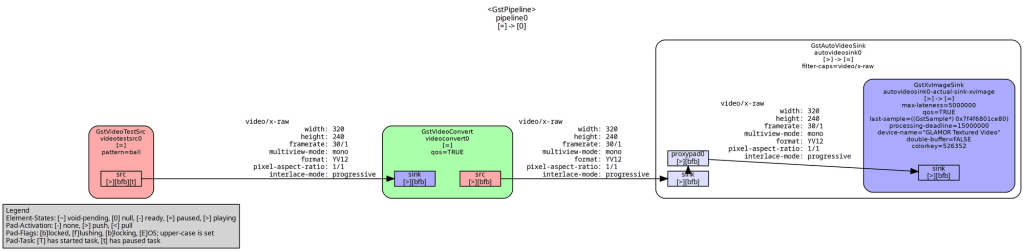
The GStreamer pipeline can be visualized using GraphViz software. Type in the console:

GST_DEBUG_DUMP_DOT_DIR=. gst-launch-1.0 videotestsrc pattern=18 ! videoconvert ! autovideosink

It will create a number of .dot files in the current directory (‘.’). Choose the one named “….PAUSED_PLAYING.dot”. The result is shown in Fig. 2 (such figures tend to be cluttered with details).

Fig. 2. A GStreamer pipeline visualized by GraphViz.

Branched Pipelines

You can create branched pipelines in GStreamer. The first type of branching happens when you duplicate a data stream with the tee element:

gst-launch-1.0 videotestsrc ! videoconvert ! tee name=t ! queue ! autovideosink t. ! queue ! autovideosink

It creates two windows with identical videos. Note how we name the tee element as t (any name could be used instead of t, e.g. cyberdemon), and then put space and not ! after autovideosink (no linking), then start another branch with t. (go back to the element named t, and try to link its other still unlinked pad). This pipeline is shown in Fig. 3.

Fig. 3. A branched pipeline visualized by GraphViz.

Another type of branching happens if an element has two or more source (output) pads with different media tracks. For example, let’s take high level decoding elements decodebin and uridecodebin. They behave similarly, except that decodebin receives data from a sink (input) pad, while uridecodebin receives data from a URI. So the two lines are very similar

uridecodebin uri=<file name>

and

filesrc location=<file name> ! decodebin

except the first one requires a full path. Let’s try to play a media file with uridecodebin:

gst-launch-1.0 uridecodebin uri=file:///home/seymour/Videos/suteki.mp4 name=u ! audioconvert ! audioresample ! autoaudiosink  u. ! videoconvert ! autovideosink

Once again, you have two branches after uridecodebin:

uridecodebin ! audioconvert ! audioresample ! autoaudiosink
                        ! videoconvert ! autovideosink  !

This pipeline behaves similarly to playbin. uridecodebin is a high-level element, which automatically creates a sub-pipeline with appropriate demuxer and decoders.

Can we go to a really low level? Yes, but there is usually no need to. We can inspect our file with gst-discoverer-1.0 or ffplay. If we know that suteki.mp4 is a QuickTime file with AAC audio and H264 video, we can then play it with:

gst-launch-1.0 filesrc location=suteki.mp4 ! qtdemux name=d ! avdec_h264 ! queue ! videoconvert ! autovideosink d. ! avdec_aac ! queue ! audioconvert ! audioresample ! autoaudiosink

Here the two branches are:

filesrc  ! qtdemux ! avdec_h264 ! queue ! videoconvert ! autovideosink

                               ! avdec_aac ! queue ! audioconvert ! audioresample ! autoaudiosink

We see demuxer and decoders, and a new element queue. Note that the queue in GStreamer is called queue, while the word “buffer” means something completely different (I’ll get back to it eventually). It’s always a good idea to use queue in branched pipelines to avoid a possible deadlock, when synchronizing tracks on playback or especially muxing, as GStreamer does not check for deadlocks. 

Now let’s try encoding. Now you have no choice but to go to the low level: encoders+muxer, sometimes also parser.

Video:

gst-launch-1.0 videotestsrc ! videoconvert ! x264enc ! avimux ! filesink location=out.avi

gst-launch-1.0 videotestsrc ! videoconvert ! x265enc ! h265parse ! matroskamux ! filesink
            location=out.mkv

gst-launch-1.0 videotestsrc ! videoconvert ! vp9enc ! webmmux ! filesink location=out.webm

Audio:

gst-launch-1.0 audiotestsrc ! audioconvert ! wavenc ! filesink location=out.wav    

gst-launch-1.0 audiotestsrc ! audioconvert ! lamemp3enc ! filesink location=out.mp3 

gst-launch-1.0 audiotestsrc ! audioconvert ! vorbisenc ! oggmux ! filesink location=out.ogg 

gst-launch-1.0 audiotestsrc ! audioconvert ! avenc_wmav2 ! asfmux ! filesink
          location=out.wma 

And now the hardest case. Let’s decode and re-encode:

gst-launch-1.0 filesrc location=zoryana.webm ! decodebin name=d ! queue ! audioconvert ! avenc_aac ! avimux name=m ! filesink location=out.avi d. ! queue ! videoconvert ! x264enc ! m.

What was that? A pipeline with splitting and merging branches!

filesrc ! decodebin ! queue ! audioconvert ! avenc_aac ! avimux ! filesink

                                 ! queue ! videoconvert  ! x264enc    !

Pipeline Tricks, GStreamer Real-Time vs. Offline Pipeline

There are a couple of extra tricks when designing pipelines. If there are multiple pads, the first suitable one is linked. This is not always desired. We can specify the pad name explicitly for linking, but only if we know the pad’s name, e.g. video_0 in demuxers:

gst-launch-1.0 filesrc location=zoryana.webm ! matroskademux name=d d.video_0 ! vp9dec ! videoconvert ! autovideosink

The second trick is the caps filter. If we write caps instead of an element between the two ! signs, then we force the negotiation process to only accept caps compatible with the specified caps. We can often use it to control elements that we cannot control directly, for example:

gst-launch-1.0 videotestsrc ! video/x-raw,format=BGR,width=1024,height=768 ! videoconvert ! autovideosink

Here the caps filter affects the negotiation between videotestsrc and videoconvert. videotestsrc cannot be programmed directly, but it is rather flexible at negotiations, and here we force it to produce 1024×768 BGR video. Similarly, It can be used to explicitly control the conversion elements, if we want to convert the media into a different sampling rate, frame size etc. Later we will work with appsrc and appsink. They can be configured with either direct caps (preferred) or a caps filter.

The final trick is the sync option, present in most sinks, including autovideosink and appsink. Try the following pipeline:

gst-launch-1.0 filesrc location=suteki.mp4 ! decodebin ! videoconvert ! autovideosink sync=true

This is the default. sync=true means that autovideosink plays the video stream at the 1x speed, provided that it has correct timestamps, actually in this case autovideosink sets the pace of the entire pipeline, as decodebin could decode the file much faster on modern computers. This is the GStreamer way of creating a real-time pipeline.

Now try to change to sync=false and see what happens (laughing smiley) !

If, on the other hand, we used a filesink, like in the re-encoding example above, it has sync=false by default. The pipeline plays as fast as it can (depending on processing speed), usually much faster than 1x. This is the offline file processing, GStreamer way.

The sync option is important for appsink, depending on our computer vision application, both choices make perfect sense.

In this section, I will cover a few topics which are neither “GStreamer in terminal” (previous section) nor “GStreamer in C/C++” (next section).

Does OpenCV Use GStreamer? A Tricky Relationship between the Two Libraries

Remember, I promised to explain why OpenCV, a popular computer vision library, is not good for reading and writing video files with VideoCapture and VideoWriter respectively. First, and this is the main reason, OpenCV cannot work with audio tracks at all. Second, it is rather inflexible, for example, try to encode into memory and not a disk file, you cannot! Third, depending on how OpenCV is built, it might have very limited codec support or none at all. There are no guarantees. For example, on modern Ubuntu, apt-installed OpenCV (for C++) is pretty good, while pip-installed Python OpenCV has very limited encoding capabilities.

How does OpenCV work with videos? It uses various backends, which at least for Linux usually means (surprise, surprise) either FFmpeg or GStreamer. And a couple of years ago Ubuntu switched from FFMpeg to GStreamer (1:0 for the latter !). If you are using OpenCV video I/O, you are actually using FFmpeg or GStreamer, why not cut the middle person?

There is another topic worth mentioning here, GStreamer in OpenCV. If (and only if) OpenCV was built with GStreamer, you can use GStreamer pipeline strings instead of file names in OpenCV VideoCapture and VideoWriter, terminated with appsink or appsrc respectively. It is discussed a lot in places like Stack Overflow, however, I don’t find the idea especially good. While it can slightly expand OpenCV powers with things like RTSP, you still cannot have audio or pipelines with multiple sources/sinks or anything complicated.

A much better way to combine GStreamer with OpenCV (in my opinion) is presented in the next section. With appsink and appsrc, you can move the raw pixels back and forth between your C++ code and GStreamer pipeline. Once the frame is in your C++ code, you can do anything you want with it. For example, wrap it with OpenCV’s cv::Mat, process it with OpenCV, and send the result back to GStreamer. Or, run a neural network inference or any computer vision code you want.

GStreamer and Deep Learning

Nowadays, “computer vision” and “audio processing” very often means “deep learning”. Owing to Deep Learning (DL) popularity, a number of plugins and frameworks have been proposed to run a neural network inference within the GStreamer pipeline.

  • Nvidia Deepstream
    https://developer.nvidia.com/deepstream-getting-startedThis is an Nvidia GPU-only Video Deep Learning framework based on GStreamer. Apart from neural network inference with TensorRT, it also supports Nvidia accelerated encoding+decoding, with an option to run the entire pipeline on the GPU. It is Linux-only and requires strict CUDA and CuDNN versions, better run it in Docker if you want to try. It also runs on Nvidia Jetson devices.
  • GSTInference
    https://nnstreamer.ai/
    A GStreamer framework based on R2Inference, which supports inferences with a number of DL frameworks, such as TFLite.

Note that you don’t have to use any of these frameworks to do neural network inference, you can always move data to your code with appsink and appsrc, and run the inference yourself in your own C++ code (or even in Python code for this matter), enjoying the total programmatic control over how you do the inference and visualization.

GStreamer vs Google MediaPipe

Here I compare GStreamer to another pipeline library, Google MediaPipe. I happened to play with both libraries in C++, and previously wrote a MediaPipe article (part1, part2, part3) in this blog. Let us now compare the two libraries (this is partly my subjective experience). At first glance, the two libraries are similar, as they are both multi-thread pipeline libraries. However, if you dig deeper, you will see numerous differences.

  • Background: GStreamer is old and time-tested, part of GNOME. MediaPipe is relatively new, developed by Google.
  • Main Goal:  Rather different. MediaPipe is mostly about Deep Learning, while GStreamer is mainly about playback, streaming and re-encoding media.
  • Deep Learning:  MediaPipe can do Deep Learning with TensorFlow (Lite). It also has a number of pre-trained TensorFlow Lite-based “solutions”, and many people actually believe (completely mistakenly) that the “solutions” IS MediaPipe. GStreamer can only do DL with third-party frameworks.
  • Traditional audio and video processing (resampling, reencoding, resizing, filtering): GStreamer does these things much better and has a vast array of standard elements.
  • Languages: C with GObject for GStreamer, C++ for MediaPipe. Bindings for a few other languages are available, but you’ll need C++ to get the most out of both frameworks.
  • Platforms: All common platforms for MediaPipe, except WASM for GStreamer. However, you’ll have to build MediaPipe from the source in order to use it in C++.
  • Data: MediaPipe: handles arbitrary data, but two or three special classes are available for images and audio. GStreamer: Highly specialized for audio+video via the caps system.
  • Data formats and negotiation: GStreamer: a sophisticated caps system and a wide variety of formats. MediaPipe: very few formats and negotiation is virtually non-existent.
  • Codecs and containers: GStreamer: Pretty much all codecs and containers that exist are supported via plugins. MediaPipe: Limited support based on OpenCV + FFmpeg.
  • Video with audio tracks: GStreamer: It’s easy to read a video file and split it into audio + video data within the same pipeline, same with writing files. MediaPipe: I am not sure if it’s possible at all with standard calculators, probably not. In other words, it does not qualify as “one library to rule them all”.
  • Network streaming: GStreamer: has plugins for network streaming. MediaPipe: Does not (if I remember correctly).
  • Pipeline definition: GStreamer: text string or C++ code. MediaPipe: ProtoBuf text string.
  • Internal structure: MediaPipe is generally simpler and easier to understand and to micromanage and to write custom “calculators” (similar to GStreamer elements). For GStreamer, it is much harder to go “under the hood” and write custom elements. However, you can use apprsc and appsink, as explained in this article.
  • Timestamps and synchronization and real-time vs offline: In my opinion, MediaPipe does these things in a clearer and simpler way (offline by default), while in GStreamer default behavior depends on the sink used.
  • Queues:  MediaPipe by default uses unlimited queues at each pipeline link. In GStreamer, you have to always add queue elements manually, with a few exceptions like apprsc and appsink. GStreamer is prone to deadlocks if you are not careful.
  • Documentation and tutorials: Good for GStreamer, bad for MediaPipe. MediaPipe documentation touts the “solutions” and largely ignores the C++ API .
  • Bazel factor: MediaPipe requires Bazel to build itself AND your project and it is pretty much incompatible with the “normal” C++ world of CMake and make and apt-installed libraries. This is very inconvenient, and seriously limits the possible uses of MediaPipe. In contrast, GStreamer is easy to install (with apt in Ubuntu) and perfectly friendly to CMake and make and other build systems.

    All things considered, GStreamer is much easier to use in C++ projects due to the horrific “Bazel factor”. Otherwise, their goals and typical use cases are rather different.

Let’s Sum Up

So far, we have covered what GStreamer is, how it works, its use cases, and how to run it in the terminal. We have also explained the relationship between GStreamer and OpenCV, what options there are to run a neural network inference within the GStreamer pipeline and compared it with the Google MediaPipe library. Now, let’s do some coding – follow us to the GStreamer C++ tutorial!


Apple RoomPlan API Integration for Innovative AR Apps

How to Integrate Apple’s RoomPlan API into Your iOS App: A Comprehensive Guide

Creating a 3D room model has historically been a lengthy, costly, and error-prone process. Real estate managers wasted hours and money hiring experts to make floor plans.

But here’s what changed everything: Apple introduced the RoomPlan API

Now, users can visualize rooms using their iOS mobile devices in just minutes with incredible detail. AR app developers, proptech startups, interior design platforms, e-commerce, and real estate professionals can benefit from the RoomPlan API.

“When comparing scan dimensions to actual measurements using Apple’s RoomPlan API, they turned out to be accurate enough, with an error usually staying below 5%. This level of precision makes it viable for many professional applications, from interior design to real estate documentation.”  

– Oleg Ponomaryov, CTO at It-Jim

This guide walks you through everything you need to know about integrating Apple’s RoomPlan API into your iOS app, namely:

  • What is Apple RoomPlan, and how does it work?
  • How to integrate Apple’s RoomPlan API into your iOS app.
  • Measurable benefits from the RoomPlan API integration.
  • Overcoming RoomPlan API limitations with proven workarounds.
  • Advanced use cases powered by It-Jim.

Let’s start by understanding how the Apple RoomPlan API works and its core properties.

What is the Apple RoomPlan API & Its Workflow?

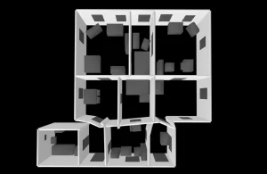
Apple’s RoomPlan API is a framework that uses augmented reality (AR) and the LiDAR Scanner on iPhone and iPad to create 3D models of indoor spaces. This is part of ARKit for building AR apps and using the RoomPlan API.

LiDAR stands for Light Detection and Ranging and uses laser light to measure distances. The technology sends out beams and checks their reflections. RoomPlan API in iOS creates a parametric model that shows the positions and sizes of walls, doors, windows, furniture, and other appliances.

The RoomPlan functionality facilitates automatic object recognition, real-time 3D model reconstruction, and enables easy exports.

Here is a list of potential use cases of an AR app containing the Apple RoomPlan API:

  • Real estate: create virtual tours of properties and provide accurate floor plans.
  • Architecture: preview and change room layouts in real-time for faster design decisions.
  • Interior design: visualize how furniture fits in a room and plan renovations.
  • Facility management & Logistics: plan office layouts or maintenance paths, inventory space usage in commercial buildings
  • Home repair: estimate material needs for renovating projects and visualize the results.
  • Accessibility: help assess room layouts for mobility aids (e.g., wheelchairs), simulate navigation paths for accessible design compliance
  • Furniture retail: allows customers to visualize furniture in their homes.
  • Marketing: create engaging advertisements or digital promotions.
  • Insurance: provide accurate documentation of property layouts and valuable items used for insurance underwriting or claims processing.

Also, RoomPlan’s ability to generate accurate 3D models of indoor spaces makes it well-suited for emergency planning, evacuation modeling, and risk assessment in occupational safety contexts.


Thinking about building a custom AR app and integrating Apple’s RoomPlan API for your business?

Whether you’re building AR apps, using the RoomPlan API to visualize spaces, or creating digital property twins, unlock faster, more innovative development. We don’t just use RoomPlan API – we help enhance it with computer vision services. Reach out to ask questions and receive advice.

Feel free to contact us.


Why Apple’s RoomPlan Outperforms Traditional Methods

RoomPlan API in iOS outperforms older methods, such as Scene Reconstruction and manual CAD modeling. It offers faster results, better accuracy, and greater accessibility, all from one mobile device. Traditional 3D scanning produces unstructured point clouds or meshes.

In contrast, RoomPlan API generates a semantic understanding of interior spaces. Instead of just capturing shapes, it identifies and categorizes room elements. The API produces this comprehensive room data within minutes.

Additionally, previous methods required extensive technical expertise, specialized equipment, and considerable post-processing time. 

How Does the Apple RoomPlan API Work?

The process for using the RoomPlan API is straightforward: launch the app, follow the steps to scan the room, and review the results shortly thereafter. You can access and edit the 3D room model anytime.

Making a 3D room reconstruction with Apple RoomPlan API

So, how does Apple RoomPlan API work from a technical perspective?

In brief, the API workflow consists of these three main steps:

1. Scanning

The RoomPlan API uses the device’s camera and LiDAR scanner. It captures the environment and identifies key features: walls, windows, doors, and openings.

2. ML Processing

Sophisticated ML algorithms analyze the captured data to identify room features and create a 3D model of the room. 

3. 3D Output

The RoomPlan API in iOS gives results as parametric data. You can export this data in different Universal Scene Description (USD) formats. This property enables developers to easily add 3D models to their apps.

USD is a typical format for AR-based projects. You can edit these files later in tools like AutoCAD, Shapr3D, or Cinema 4D if needed.

RoomPlan API: Data Structure Overview 

Apple’s RoomPlan can recognize the following aspects of the captured room

  • Structural elements: walls, doors, windows, openings.
  • Furniture: chairs, tables, sofas, beds, storage units.
  • Room boundaries: floor plans, room dimensions.
  • Spatial relationships: object positioning and room layout connections.

Now, let’s see what data is contained in the 3D model produced by the technology. RoomPlan organizes scanned information into two primary categories: surfaces and objects.

3D model scan of the larger room with more furniture

4 Surface Types & Their Data Properties

First, let’s elaborate on surface types, properties, and applicable metrics. RoomPlan identifies four distinct types of surfaces that define a room’s structural boundaries:

  1. Wall – primary structural boundary.
  2. Door – entry and exit points.
  3. Window – light sources and viewing areas.
  4. Opening – passages without doors.
Surface Type Description Detection Capability Relevance
Walls Vertical structural boundaries Precise positioning and dimensions Structural layout for AR navigation and space planning
Opennings Doors, windows, passages Type identification and measurements Traffic flow analysis and accessibility planning

Useful for layout planning, renovation

Floor Horizontal base surface Area calculation and boundaries Foundation for furniture placement and room use
Furniture Moveable and built-in objects Category, size, and spatial relationships Object interaction and interior design applications


Each of these surfaces contains a standardized set of six data properties. 


Data Property Description Data Type Notes
Confidence Detection reliability Discrete (Low/Medium/High) Indicates scan quality
Dimensions Size measurements Width × Height Depth always equals 0 (no thickness)
Transform Position and orientation 4×4 matrix Standard transformation matrix
Normal Surface direction 3D vector Perpendicular to the surface plane
Curve Surface curvature Variable/nil Nil for flat surfaces
Completed edges Scan completion status Array Tracks user scanning progress

15+ Objects & Data Properties

Apple RoomPlan API can detect a variety of objects, namely:

  • Furniture: bed, chair, sofa, table.
  • Kitchen appliances: dishwasher, oven, refrigerator, sink, stove.
  • Bathroom objects: bathtub, toilet, washer, dryer.
  • Other: fireplace, stairs, storage, television.

Objects share similar properties to surfaces but with key differences. 

Property values include confidence, dimensions, and transform.

  • 3D Dimensions: Full width × height × depth values.
  • Oriented Bounding Boxes: Match object orientation, not world coordinates.
  • Spatial Relationships: Position relative to walls and other objects.

Dimensions and the transform metric define a bounding box around an object. The bounding box isn’t aligned with the axes. Instead, it matches the object’s orientation, not the world coordinate axes.

Data Property Description Object vs. Surface Difference
Confidence Detection reliability Same discrete values (Low/Medium/High)
Dimensions Size measurements 3D values (width × height × depth)
Transform Position and orientation Defines a non-axis-aligned bounding box

As understood, RoomPlan API can detect and visualize many elements. Additionally, it cannot simply be visualized as plain boxes; however, you can replace them with real furniture models to make the scan more detailed and valuable.  

This structured method makes RoomPlan data ideal for creating top-notch AR apps, architectural analysis, and automated space planning.


Want to explore how the RoomPlan API can transform your project?

Let’s build a solution that goes beyond the RoomPlan API’s standard features and addresses its limitations. This custom solution creation uses an advanced computer vision algorithm. It enhances object recognition and layout accuracy, especially in cluttered or irregular rooms.

Reach out for a consultation.


Getting Started with the Apple RoomPlan API: Tech Perspective 

Developers can seamlessly use the RoomPlan API in their iOS apps using one of two approaches:

  • Basic integration: add a RoomPlan API with minimal effort and without customization. Users will interact with the built-in solution experience only.
  • Advanced integration: gain complete control over scanning parameters and real-time data processing. From this perspective, users can build detailed room plans and edit specific elements as needed.

Thus, the easiest way to integrate Apple’s RoomPlan API into your iOS app is by using the default RoomCaptureView in Storyboard.

RoomPlan follows a clear component hierarchy: 

Hierarchy of components included in RoomPlan API


The most straightforward integration uses the default RoomCaptureView for Storyboard.

  1. The RoomCaptureView handles all visualizations and interactions with the end user. 
  2. A user scans the room with RoomCaptureSession, accessed via the corresponding view’s property. 
  3. The RoomCaptureSession itself utilizes the standard ARSession from ARKit.

You might also find it interesting to read:

SDK for Augmented Reality Applications

How Do AR Solutions Benefit from RoomPlan API

When building AR apps and using the RoomPlan API, focus on how to streamline your business processes. 

According to Statista, revenue in the AR&VR market is expected to reach $46.6 billion in 2025. Companies are investing in AR technology because customers want to receive immersive and interactive experiences in their services.

Integrating Apple RoomPlan into your app improves development and user experience in several key ways:

  • Reduce software development time by more than 50% with this unique iOS technology.
  • Generate 3D floor plans in under 2 minutes.
  • Offer intuitive room capture in real estate, interior design, or AR apps.
  • Cut the need for specialized 3D modeling expertise on your team.


“RoomPlan integration cuts our MVP development cycle from 4 months to 6 weeks. We could focus on user experience and advanced functionality instead of building a scanning solution from scratch.” 

– Yurij Gapon, Head of iOS at It-Jim

We can help you test the RoomPlan API integration in your project and ensure accuracy in real-world conditions, such as varying lighting and complex furniture setups.

You can also discover our

3D Computer Vision Services


The true strength of using the Apple RoomPlan API is not only in its scanning features. It also provides valuable business insights.

Here’s how RoomPlan translates technical capabilities into competitive advantages:

1. Faster Time to Market

Scan-based 3D room models eliminate the need for manual drawing, significantly speeding up product release timelines. 

Teams can now iterate and deploy features in just days. There is no need to wait weeks for professional architectural drawings. There is no need to use CAD programs and similar tools and to hire an external expert for measurements.

2. Improved App Experience

Integrating RoomPlan into your iOS app offers an immersive AR experience, enabling engaging and personalized interactions. This creates engaging, personalized experiences. They feel real and fit into the actual environment, not just a theoretical space. 

Users interact with real-world spatial data instead of static, generic layouts. Planning renovations, arranging furniture, or evaluating properties all become easier and more intuitive.

3. Optimized Processes

RoomPlan API streamlines floor plan creation by automating the process, reducing manual effort, and minimizing errors. It’s a valuable tool for professionals who need fast, reliable, and accurate results.

4. Data-Rich Outputs

RoomPlan output provides detailed object metadata, including:

  • Type classification.  
  • Precise positioning.  
  • Accurate dimensions.  
  • Spatial relationships.

This structured data is directly integrated into analytics pipelines, AI training datasets, or modeling applications. There’s no need for extra processing.

5. Ready-to-Export Formats

The API provides seamless workflow integration with various export options:

  • USDZ files for AR apps.
  • Structured JSON for BIM/CAD tools. 
  • Standard formats for cross-platform use.

Building AR Apps with Apple RoomPlan: It-Jim Experience 

Our team has rolled out the RoomPlan API in various industries. This adoption change enables businesses to tackle spatial computing challenges in innovative ways.

Here are proven applications that we helped to implement:

Architecture: 3D Floor Plan Layout  

Project Focus: The goal was to create precise 2D floor plans and 3D layouts of real spaces with actual dimensions.

Solutions: A system captures spatial data from iPhone LiDAR scans. Then, it creates 3D models and scaled 2D floor plans.

Result: A mobile app turns spaces into digital layouts in minutes. This outcome saves architects and real estate professionals a whole day of manual work.

Solution for Real Estate

Challenge: Our solution creates 3D room models to facilitate the buying and selling of real estate. A client requested that our team enhance their prototype, which was created using the Apple RoomPlan API. They also requested support to improve app functionality.

Solution: We developed a tool that creates 3D room models to help with buying and selling real estate properties. 

Furniture Fitting AR App

Challenge: Customers struggled to see how furniture would look in their own spaces. This aspect caused high return rates and unhappy customers.

Solution: We developed an AR app using the Apple RoomPlan API, which enables users to place furniture in real-time with precise spatial awareness. Users scan their room once, then virtually place items with confidence in scale and fit.

“After It-Jim added RoomPlan to our property management platform, we cut manual surveying costs by 70% and improved accuracy. Property listings now include interactive 3D models generated in minutes, not days.” 

– Feedback from our client. 

Therefore, RoomPlan API integration makes a solid investment. The technology offers businesses chances to stand out. It helps them create a better user experience and visual materials with less effort.


Have an AR-based project concept in mind and want to use the RoomPlan API? 

Let’s build it together with Apple RoomPlan technology and advanced computer vision expertise. We help you turn powerful technology into real-world solutions that deliver results with a proven track record of implementing the RoomPlan API in iOS apps across diverse industries. 

Book a call to discuss the implementation strategy.


Overcoming Apple’s RoomPlan API Limitations 

Note that RoomPlan is still a new API. Some things may change, and issues might get fixed in future updates. 

However, RoomPlan delivers useful but not perfectly accurate results. Measurements and object positions may have minor errors, which is excellent for quick scans but not reliable for precision-oriented tasks.

Since our team has had an immersive experience with the Roomplan API, we’ve identified its key limitations and know how to work around them.

How we work with existing API limitations, read also:

RoomPlan is Awful, and it’s Great!

For example, the RoomPlan framework has significant constraints, including the requirement for rectangular simplifications. The system attempts to reduce all objects and surfaces to a set of rectangles. 

Additionally, the technology does not capture data from ceilings or skylights.

Limitation of Apple RoomPlan API examples with a window and a door

The current version of the RoomPlan API in iOS has several constraints, such as:

  • Limited object recognition – detects only a fixed set of common household items (e.g., chairs, tables, sofas). It does not identify less typical objects, such as water boilers or industrial equipment.
  • Struggles with multiple or large rooms – not designed for scanning numerous or very large spaces in one go. Apple recommends a maximum of about 9×9 m (30×30 ft). Longer scans degrade tracking accuracy, risk overheating, and may lead to drift.
  • Measurement Errors – shows measurement drift—errors up to ±5 cm per wall.
  • Incorrect Wall Thickness – models all walls as a uniform thickness of around 16 cm, regardless of real measurements. Exterior walls are always that thin; structures over ~50 cm break into two separate thin walls.
  • Door & Window Flaws – merge double doors or door-window combinations incorrectly.
  • Mirrored Surface Issues – large mirrors and mirrored wardrobes can confuse LiDAR, leading to missing geometry or phantom objects.
  • Surface shape limitations – assume surfaces are rectangular or slightly curved, so it misrepresents angled walls, arched openings, or detailed trim.
  • Phantom (ghost) geometry – occasionally “sees” surfaces or objects that don’t exist; LiDAR noise can lead to phantom walls or objects.
  • No Ceiling or skylight capture – does not capture ceilings or skylights, making it unsuitable for tasks requiring lighting design or accurate volume measurements.

RoomPlan API exteme case of scanning the whole house at once


While powerful, RoomPlan isn’t perfect in every environment. With years of vision-based R&D, we know how to work with these and other limitations.

Apple continuously improves RoomPlan API capabilities with each iOS platform update. Our AI iOS development services and approach account for this evolution.

“We are leveraging new RoomPlan features as they’re released. Our clients enjoy Apple’s upgrades while keeping current features intact. This is the benefit of working with a team that knows the framework’s roadmap and even beyond.” 

– Yurij Gapon, Head of iOS at It-Jim

Conclusion: Is Apple’s RoomPlan API Right for Your Project? 

Apple’s RoomPlan API simplifies the creation of accurate 3D room models. You can use it with a LiDAR-enabled iPhone or iPad.

It simplifies floor plan creation, reduces errors, and enhances app features across various industries, namely:

  • Real Estate: virtual property tours and instant floor plan generation.
  • Interior Design: AR-powered furniture placement, estimating materials, and space planning.
  • Retail: store layout optimization and virtual showrooms.
  • Property Management: digital twin creation and facility maintenance.
  • Architecture: rapid as-built documentation and renovation planning.
  • and much more.

Its ability to quickly generate accurate room layouts also makes it a valuable asset for broader AR applications. The technology is excellent for:  

  • Fast residential room scans within ~9×9 m.
  • Quick, parametric 3D models and object layouts.

What’s Next: The RoomPlan API is still new, but updates will improve its accuracy and stability. 

In the future, we can look forward to improvements such as support for non-rectangular surfaces, scanning multiple rooms, and better detection of floors and ceilings. These upgrades will expand the capabilities of what we can achieve with spatial understanding in AR.

Please note: The technology is not suitable for high-precision needs, complex structural analysis, industrial settings, or multi-floor scanning.


Ready to advance your business with the RoomPlan API and computer vision?

We help you benefit from the RoomPlan API. We do this by testing, customizing, and integrating it into your iOS app. Contact our team to share your needs and find out how we can speed up your RoomPlan implementation.

Writings on the Wall: Recognizing Speech on Spectrograms

If you’ve ever come close to anything related to audio or other signal processing, you likely already know about spectrograms. Those fancy-looking and usually colorful plots are commonly used to represent a spectrum’s change over time. But can they provide us with some higher-level information about, let’s say, human speech? What if I told you that one could effectively get a transcript of a speech recording just from its spectrogram? Well, if you think that this is rather an exaggeration, you’re absolutely right. Yet, recognizing certain phonemes and even making educated guesses about specific words based only on their spectrograms is perfectly possible. Thus, let’s dive deeper into this topic and learn a thing or two about human speech on our way.

Power-Source-Filter Model

A common way to represent human speech is a so-called Power-Source-Filter model. The Power here refers to the lungs where an air flow originates, vocal cords are the Source of vibrations and everything above them (the vocal tract) serves as the Filter for those vibrations.

We can ignore the Power component for our current goal and focus only on the Source-Filter part. Using more accurate terms than just “vibrations,” the Source produces harmonic waves with a fundamental frequency depending on the voice pitch. The Filter then either amplifies or suppresses specific harmonics. Peaks on the filter’s frequency response are called formants and are denoted as F1, F2, etc. (from lower to higher frequency).

The Filter is considered linear, i.e. a current sample is approximated as a weighted sum of n previous samples. Given a speech recording, one can estimate coefficients of the Filter using a Linear Predictive Coding (LPC) technique and then use them to find the frequency response curve. We need this curve (specifically its formants) to help us recognize certain phonemes.

Vowels

Phoneticians distinguish a set of 8 “cardinal vowels”, with each one being defined by a specific position of a tongue’s highest point while pronouncing it:

If we plot the highest point positions for each cardinal vowel together, they’ll form a specific figure:

If we make the same plot for frequencies of the first two formants (F1 and F2), it will look remarkably similar:

The match isn’t perfect, of course (just as my pronunciation of the cardinal vowels, from which the formants were obtained), but it is still close enough. It leads to a couple of conclusions. First, even though the model with just the linear filter might look over-simplified, it bears direct correspondence with movements of the vocal tract. Second, the frequencies of the formants (usually two or three) are unique for each vowel and can be used to distinguish them.

To observe this, we can create a plot of a speech recording that is similar to a spectrogram but with the Filter’s frequency responses used as its columns instead of spectrums. Formants on this kind of plot are seen as bright horizontal lines. If we build it for a recording of several different vowels, it is evident that formants are indeed uniquely positioned for each of them:

Let us remember this plot for a future reference and move on to consonants.

Consonants

Unfortunately, there is no unique descriptor for each consonant, unlike formants for vowels. Instead, we can categorize consonants and use this classification to narrow down a list of possible options when trying to recognize a particular phoneme.

To analyze consonants, we need to pronounce them between two vowels, which makes them better defined on spectrograms. So, all examples were pronounced with two [a] sounds, like [apa], [ada], etc.

Arguably the most important category split is voiced and voiceless consonants. While pronouncing voiced ones, vocal cords still vibrate; thus, we can observe some harmonics. During voiceless ones, the vibration is absent, and harmonics are entirely interrupted. As evident from the following plot, while all consonants do look like “gaps” between vowels, voice ones ([b] and [d]) still leave some harmonics uninterrupted:

Fricatives can be recognized by a characteristic noise. Furthermore, the distribution of the noise along the spectrum can help to distinguish them from each other:

The frequency response can be helpful for consonants too. For instance, nasal consonants have a specific noise that is better observed on this kind of plot:

Trilled consonants ([r] in this case) can be easily spotted too by a very characteristic vertical pattern:

Some other features can help recognize consonants; however, they are more advanced and often harder to spot, so we’ll leave them out of scope for now.

Reading Words

Now, when we’ve learned to recognize different phonemes, why not try to do something more remarkable, like reading an actual word from a spectrogram? Here is one, with its spectrogram and corresponding frequency response plots:

We can immediately identify three separate vowels. Just by looking at the reference of different vowels that we’ve prepared earlier, we can pick the ones that look the most similar:

The second noticeable thing is three fricatives that can be identified by their noise using another reference from earlier:

Now we have just three missing phonemes. The first one can be easily recognized on the frequency response plot as a trilled consonant, with [r] being the only possible option in English. The second one is somewhat hard to identify, so we’ll skip it. Finally, the last missing one can also be identified on the frequency response plot as a nasal consonant (either [n] or [m]). So, here are our final predictions:

We still have one unknown consonant and ambiguity regarding another one, yet what we’ve discovered is enough to “brute force” the word, which is obviously “frequency”.

Conclusions

So, we’ve learned to recognize some phonemes on spectrograms. That is something you could brag about to a very limited number of people who would actually consider it cool but are there any practical applications to all this knowledge?

First, if you’re building any kind of speech processing pipeline with spectrograms as its inputs, you now know about features to look for and can tune spectrogram parameters to highlight them better. Or you can even use frequency responses for additional features. Also, if you have a speech-generating model (especially a black box one, like a neural network) and its output sounds wrong, you could compare its spectrogram to an actual speech and try finding the source of your troubles. And finally, what we’ve discussed in this post is present in many classic speech processing methods. Linear Predictive Coding, for example, is used for voice compression (like earlier versions of GSM), speech synthesis, speech encryption, audio codecs, etc. And it is always good to know the basics, even when working with much more advanced stuff.

Computer Vision in a Web Browser: Practical Examples

This blog post covers some important aspects of deploying and running classical computer vision algorithms as well as convolutional neural networks in a web front-end. Please make sure you have read the first part of the blog post. This will definitely help you to follow all technical aspects much easier.

Emscripten for Computer Vision

How can you pass an image or a video frame from JS to C++ and back? We’ll give a minimal example. Suppose you have an image in an <img> tag. First, you have to copy it to RGBA pixels (only RGBA format is supported, not RGB !) via a <canvas> tag:

const img = document.getElementById('myImg');
const canvas = document.getElementById('myCanvas');
const ctx = canvas.getContext('2d');
const w = img.width; const h = img.height;
canvas.width = w; canvas.height = h;
ctx.drawImage(img, 0, 0);
const data = ctx.getImageData(0, 0, w, h).data; // Uint8ClampedArray
const bSize = data.byteLength; // == 4*w*h

Next, you have to send the Uint8ClampedArray object data to C++. However, C++ cannot access JS objects directly (at least, not efficiently). They are not part of the C++ memory, which itself is only a part of the JS memory. Some copying is unavoidable. Let’s copy data to the C++ heap:

const dataPtr = Module._malloc(nBytes); // C++ malloc
const dataHeap = new Uint8ClampedArray(Module.HEAP8.buffer, dataPtr, nBytes);  
dataHeap.set(data);  // Copy data -> dataHeap

Here dataHeap is a view object for the C++ data.

Now we can finally call the C++ code to do something to the image. We pass dataPtr, a pointer to data on the C++ heap. No result is returned here, but the image can be modified in-place:

Module._process(dataPtr, nBytes, w, h);

Finally, let’s show the result on the canvas and free the C++ buffer:

ctx.putImageData(new ImageData(dataHeap, w, h), 0, 0);
Module._free(dataPtr);

It’s very important that C++ has no garbage collections, so if you use malloc(), you must free() afterwards, otherwise there is a memory leak! Memory leaks are extremely evil. You might not notice them in a minimal demo, but they will kill a real project.

Emscripten and OpenCV

Traditional CV algorithms in C++ typically use OpenCV. Can we build it with emscripten and use it in our custom C++ projects? Yes, but with a few caveats. 

First, the emscripten build of OpenCV uses a custom build script build_js.py. Unfortunately, it’s made for an ancient emscripten version (2.0.10) and doesn’t work with modern ones. You have two choices. You either use version 2.0.10 and miss the features and optimizations of modern emscripten versions; or hack the build script to make it modern-version compatible, which is not easy. 

Second, this build script builds Asm.JS by default; you will have to specify the –build_wasm option for a WASM build, this is important.

Third, we are not sure this build is optimal. In particular, it is probably single-thread. You can dig into this stuff if you want, but it is not going to be easy.

Once the build process is finished, you will have a build directory with a lot of useful stuff, like lib and include directories, and also .cmake files. Ignore bin/opencv.js; we are not going to use that. You use OpenCV in your C++ code just like you would on a desktop platform. In particular, cmake is able to find OpenCV with find_package(), provided that you specify the option -DOpenCV_DIR=<path>, where <path> is the full path to the OpenCV emscripten build directory (the one with .cmake files). You can pass RGBA images to C++ as explained above and convert them to a cv::Mat inside your C++ code. 

But what can you do with opencv.js? First, it cannot be used in any way from your custom C++ code, thus it is pretty useless from where we stand. Second, the file opencv.js is the project of the same name (OpenCV.js), which exports a number of OpenCV functions and classes to be used directly from JS (probably via embind or something similar). As it happens, the emscripten C++ build of OpenCV (the lib directory), the thing that we want, is merely a byproduct of OpenCV.js build process from the point of view of the OpenCV team. The official OpenCV documentation does not even mention C++ emscripten usage, it presents OpenCV.js only. Calling opencv functions from JS is not very interesting from our point of view, plus OpenCV.js is inconvenient and poorly documented compared to OpenCV C++ or Python API. It’s much more interesting to build CV C++ algorithms in emscripten. Such C++ algorithms, if written well, are cross-platforms, and can be developed on desktop and later ported to mobile, front-end or embedded.

Is it possible to have both? Can we create a custom C++ code, which also exports some OpenCV stuff like cv::Mat to JS? Probably yes, with some effort, but for beginners it is much simpler to call OpenCV stuff from C++ only, and pass images from JS to C++ and back as explained in the previous chapter.

How slow is OpenCV emscripten, compared to desktop OpenCV on the same computer? It depends on the OpenCV function, but here is an example. We run Lucas-Kanade sparse optical flow cv::calcOpticalFlowPyrLK() for 400 points, and the same parameters, on the same laptop both on desktop and web browser. Our results:

    Native C++ (desktop)           WASM, Chrome   WASM, Firefox
~ 1 ms ~ 24 ms  ~ 90 ms

24-90 times, not a small difference! That is what we meant before about “custom algorithms being slow”!

Disclaimer: This applies to the default opencv WASM build with emscripten 2.0.10. It is probably single-thread. A better optimization is likely possible if you really dig into the problem, but it’s far from trivial. As a result, the web browser on your modern computer is slow ‘Like Raspberry Pi 1’ as far as CV algorithms are concerned, thus only the most lightweight ones can be successfully deployed in a web browser.

Deep Learning in a Web Browser

Nowadays, CV is mostly about neural networks, at least if you get your information from blogs and youtube channels. Can you deploy neural nets in a web browser? And how efficient is it? Short answers are: “yes”, and “very inefficient”. 

All serious neural nets use GPU (or sometimes TPU). Can a web browser use GPU? Yes, but only in the form of WebGL (web OpenGL) and not CUDA. You probably have never heard of neural networks using OpenGL on desktop, only CUDA, right? Do you wonder why? The answer is obvious: OpenGL is made for 3D rendering, not numerical calculations, and is very inefficient for neural networks compared to CUDA (on the same GPU). You’ll see some examples below. Likewise, CPU inference (in WASM) is slower than the machine-native CPU code.

Which DL frameworks are available for the web browser? We know two: TensorFlow.JS (Google) and ONNX Runtime Web (Microsoft). Both frameworks support webgl (default) and CPU inference.

TensorFlow.JS is “TensorFlow for the web”, with a JS API similar (but not identical !) to python TF+keras. It has its model format (BIN+JSON), different from TF and Keras models. It is a relatively heavyweight library with lots of utilities. Apparently, you can even train networks in a browser.  Needless to say, when we first looked at TensorFlow.JS, we were somewhat surprised. We expected a minimalistic TFlite (like on mobile platforms) but instead found something heavyweight and completely original. TFlite API also exists for the web, but if we are not mistaken, it requires full TF.js anyway. Supposedly TF and Keras models can be converted to TF.js format, but it does not always work in practice; plus we had to edit the JSON file by hand to make anything work. 

The good thing about TF.js is that it has a lot of auxiliary stuff. For example, you can create tensors from HTML <img> and <canvas> elements (automatically converting RGBA to RGB !). You also have a numpy-like tensor algebra which you can use for operations like normalization, image resize, or data type conversion. The problematic thing is that in TF.js (when using WebGL), you have to release all tensors by hand (tf.dispose()) or with the special wrapper tf.tidy(), otherwise you’ll get a catastrophic GPU RAM leak!

The other framework ONNX Runtime Web is pretty much the opposite. It is small, compact, minimalistic, and only supports ONNX format. It is good for deploying PyTorch networks (and nowadays, almost all modern neural nets are in PyTorch), as most PyTorch networks can be converted to ONNX, but not every ONNX can be further converted to TF. ONNX Runtime Web does not have tensor algebra, so you will have to implement all auxiliary operations (normalization, type conversion, RGBA->RGB) yourself (in pixel-wise JS loops) or use some other libraries.

The worst thing about ONNX Runtime Web is that it does not work. Or, rather, the original version 1.8.0 does (and the older ONNX.js), but all subsequent versions do not. The bugs are somewhere in WebGL shaders, since WASM inference works correctly. For some networks, the result is OK (e.g., torchvision ResNet 50), but for others (ResNet 18), it is completely crazy! What is the big difference between ResNet 50 and 18? Unfortunately, we didn’t have time to investigate deeper.

The most amazing thing is that several ONNX Runtime Web versions were released after 1.8.0, and they are all broken. Did nobody notice it?

For both frameworks, there is a common WebGL issue. It takes a long time to compile WebGL shaders. Thus, the very first “warm up” inference can take a few seconds. The following ones are fast, but only if the input tensor size does not change. If the network has a dynamic-sized input and the input size changes, the shaders will be recompiled. This issue is unavoidable, but a clever web developer can mask the webgl warmup with web page loading or something like that.

Finally, the speed. While we did not perform any formal test, here is what we got very roughly on the laptop with GeForce 1660 GPU (Note: unlike CPU and CUDA, WebGL inference times fluctuate wildly, even after the warmup), all on ResNet 50 from either torchvision or Keras. 

  PC
Browser (FireFox)
CUDA CPU WebGL WASM
Keras 90 ms
PyTorch 5.5 ms 60-70 ms
ONNX runtime 15 ms 50-350  ms 1000 ms
TFJS 260 ms

*Timing per one inference.

From what we see, WebGL (GPU) inference in a browser is about 15 times slower than native CPU, and about 50 times slower than CUDA. Speaking of the native CPU, ONNX runtime is way faster than PyTorch or Keras; we did not previously know that. These numbers mean that only relatively lightweight neural networks can be successfully executed in a browser unless you want inference time of many seconds.

Besides, there is a question of neural network size (the total size of their parameters in e.g. PTH or ONNX file). Modern neural networks are typically hundreds of megabytes or even gigabytes in size. The largest size practical for the front-end is perhaps about 20 Mb if you don’t want your webpage to load forever. Such super-small models are not easy to find. Please don’t expect to deploy a model from some 2022 state-of-the art paper in a web browser!

Other Technologies in the Web Browser

We’ll mention very briefly a few other web technologies which can be relevant to CV.

WebGL is available for 3D graphics, and it’s one of the “fast” technologies. Few people, however, would want to use WebGL directly. There are several convenient 3D graphics libraries that use WebGL, the most popular is Three.JS. Even Unity engine is available for the web (as an official Unity platform), based on WASM + WebGL.

WebXR is available for VR and AR (the previous specification WebVR has been deprecated and removed). But you cannot try it on your PC. WebXR requires an actual VR device, like Oculus Quest 2. On smartphones, it can do VR by showing two images on the screen, which can be viewed in 3D if you have a VR headset for your phone. Finally, it can do AR on your phone (no additional headsets required), but only if you have ARKit/ARCore, and still not all phones in existence have those. Maybe in a year or two, it will become widely available.

To Web or Not To Web?

Finally, we are ready to give the final answer to the question, “Should you put the CV algorithms on the front end?”. The answer may be different. If your CV algorithm is really lightweight, you can run it in a web browser. Otherwise, be ready for playing with your favorite neural net or heavy custom pipeline. It is much more efficient (10-50) times to run stuff on a native platform (Intel, ARM) compared to the browser. Thus, you need to always consider writing mobile applications or at least client-server web ones to control the distribution of the computational resources for heavyweight CV algorithms.

Can things get better in the future? Will the “native” and “web” worlds somehow converge?

On one hand, there are big challenges. Flashy demos for some new “fast” technologies can look very cool, but, as explained above, if we want original CV stuff, we need to write custom algorithms, which are in the “slow” category. And it is likely that WASM will always be slower than the native CPU. Neural network inference in the web browser is currently very slow compared to the native platform, but this can be easily fixed by creating new web technologies (think e.g. native-CPU ONNX runtime built into all browsers). On the other hand, browser platform is very important for rather popular Metaverse and the extended reality (XR) concepts, thus there is a strong motivation for improvement.

The world of the web tends to develop slowly (adoption of new web specifications take years), but it is likely that web browser will become a mature platform in the long term (10-20 years). We are cautiously optimistic about it.

Computer Vision in a Web Browser: Basics

Are you interested in Computer Vision (CV)? Probably yes, if you are reading this. If you read CV tutorials, you might have noticed that most of them are in Python. This applies to both traditional CV (without neural networks) and, even more, to deep learning (neural networks). Occasionally, CV tutorials use C++ instead of Python, but any other programming languages are very rare. The fact is, Python is known as THE language for research and development, math, CV, ML, DL, education, and a quick prototyping.

But what if we want to deploy our CV algorithm somewhere, i.e., to use it in real life? Then very often we will find python impossible or very difficult to use. C++ is better: it is available almost everywhere. Android and iOS platforms have their own languages: Kotlin/Java and Swift/Objective C, respectively, while Web Browsers have JavaScript (JS). But all three platforms (Android, iOS and Web) can integrate C++ code as well.

This article will introduce Computer Vision in a web browser for dummies. Note: we are talking specifically of web browsers (front end), not web servers (back end)! First, we want to run a C++ code in a browser, in particular a C++ code that uses the OpenCV library, the most popular tool in the computer vision community. Second, we want to run some neural networks in a web browser.

Disclaimer: Our background is in CV and ML, not web development. We might still be missing some technical details on the web side of things. And we deliberately skip many topics which belong to the “pure front end” and not CV, such as JS modules, bundlers, frameworks, DOM model, etc. However, minimal knowledge of JS and front-end development will definitely help you understand this article better.

CV in Front-End or Back End?

Before we start, there is an important question. Should we run CV algorithms in the front end (browser) or the back end (server)? The back end can give you much higher computational power. But you’ll pay for it, and if a million users use your website, the cost adds up quickly. If you want to take the back-end approach, there are other things to consider.  

The first is latency (delay). It often takes time for the data to travel through the internet, often up to half a second or even more. There are both physical reasons for the latency, like the finite speed of light (especially relevant for satellite connections), and other reasons, like the large number of switches and routers which retranslate your signal (never instantly). This is usually not a problem when you want to process a single image. Video is another matter. The latency doubles if the signal has to go two ways (from browser to server and back). Add to this the latency of the algorithms themselves (on the server), and you can get a pretty noticeable delay (e.g., of the order of a second), which will make your beautiful web application not so beautiful anymore.

The second problem is video streaming. Many people think it’s trivial, but it’s not. Web browsers are not made for streaming. Especially not for real-time streaming. 

But wait, what about YouTube or Netflix? It is not the same at all. They are not real-time (in fact, with quite a lot of buffering) and go one way from server to browser. Basically, the only “good” streaming option for the browser is WebRTC, but it’s made for browser-to-browser P2P connections and is extremely painful to implement on the server side. It also thinks in terms of “streams” and is not very friendly to any CV algorithms processing video frame-wise. Other options like WebSockets are much more server-friendly and programmer-friendly. Still, they use very inefficient video codecs like MJPEG (since they cannot access the built-in video codecs of the browser). And finally, two-directional video streaming can be simply problematic on slow networks due to the network load.

CV in the front end has its downsides. As we’ll see below, a web browser is simply not a powerful enough platform for heavyweight algorithms. It is especially true for neural networks. Typical modern neural networks are both too large (hundreds of megabytes) and too slow to be deployed in a browser.

To summarize this chapter:

  • For heavyweight algorithms, there is no choice: back end.
  • For processing a single image (e.g., applying effects to a photo), back end is OK.
  • For real-time video processing, it’s very hard to create a working solution with a back end, use the front end if possible.
  • Desktop or mobile apps utilize your hardware much more efficiently than the web browser, giving you 10-100 times more power (see examples in the following chapters). 

Web Browser as a Virtual Platform

While you probably did not think about it, a web browser is a platform, much like Android, iOS or Raspberry Pi. But it runs on your PC or phone, so it is a virtual device on your host system, which can be compared to an Android emulator or perhaps some PlayStation or Nintendo emulator. Web Browser would NEVER run a third-party machine code of your host machine architecture (Intel or ARM), except in browser plugins, which seem to be dying out nowadays. Instead, it has a virtual engine, or actually, more like two virtual engines (for modern browsers): JS engine and WASM engine.

JS engine runs JS code natively, without a compiling step (actually, there is a JIT compiling and many optimizations under the hood). The other engine is WASM (for WebAssembly), a machine code type. C++ and other languages can be compiled into WASM and executed in a web browser. However, WASM is not the machine language of your host. Thus, the same C++ code runs many times slower in a web browser than the same C++ code built for the host and always will in the future. By the way, if you ever hear of something called “Asm.JS,” just ignore it; it is deprecated since WASM was introduced.

As a virtual platform, the Web Browser has a lot of artificial limitations, motivated mainly by web security. Compared to other platforms (desktop, mobile, Raspberry Pi, etc.) it is probably the most painful platform to develop for.

  • You cannot access your host file system. Files can be accessed only via file chooser dialogs.
  • Many things, including the camera, require HTTPS. HTTPS is only possible if you have a certificate. 
  • Cannot autoplay videos with sound.
  • Mobile browsers have no console, and a localhost server is typically not available; thus, developing and testing for mobile browsers is much harder compared to desktop ones.
  • Cannot access different remote servers freely due to CORS issues.

Browsing Fast and Slow

One can say that a web browser turns your latest expensive PC or phone into a Raspberry Pi 1. However, it’s only half true. Some things are pretty fast in a browser. These are the things implemented as a part of the browser code itself, written in C++ and well-optimized. In contrast, any custom code of yours, whether in JS or WASM, will run pretty slowly.

Fast (or at least reasonably fast) operations, built-in into the browser:

  • Image operations using <img> and <canvas> tags, including JPEG and PNG codecs.
  • Video and audio operations using <video>, <audio> tags, including a number of codecs.
  • 3D graphics with WebGL.
  • Audio/Video streaming with WebRTC.
  • Presumably (but I didn’t test myself) WebXR.

Slow: Any custom algorithms written by you, or part of third-party JS or C++ libraries:

  • Any custom code in JS.
  • Any custom code in WASM (usually compiled from C++).
  • It includes OpenCV operations.
  • Neural Network inference.
  • Any JS library, installed by NPM or otherwise.
  • Any cross-platform C/C++ libraries compiled to WASM, like ffmpeg.js.

The fast operations are regularly advertised and showcased in beautiful demos. However. In real life, if you want to create something original, fast operations are often not enough. At some point, you will have to write your own custom algorithms in either JS or C++, and they will be very slow.

The fast operations tend to be extremely restrictive, often surprisingly so. Take for example the <video> tag. It is probably something like the combination of VideoCapture and VideoWriter of OpenCV, right? Nope! In fact, the <video> tag is almost useless for CV applications for the following reasons:

  • It cannot break the video into individual frames (no “next frame” callback).
  • Seeking a given position is supposed to exist but does not seem to work on Chrome.
  • It is strictly real-time and cannot wait while you process a frame (you cannot process a video file slowly). 
  • It cannot encode a sequence of frames into a video stream.

Basically, the <video> tag is good at only one thing: showing a video in your browser. Not for CV. WebRTC, by the way, has similar limitations and can hardly be connected to any front-end CV. What to do then if you want to process a video? None of the options are perfect, but still:

  • You can try to use the <video> tag anyway, but you might lose frames and have an irregular FPS with possible non-deterministic outputs. 
  • A library ffmpeg.js can be used, but it’s a part of the “slow world”, heavyweight and complicated.
  • New WebCodecs API as an option, however  it’s still not widely supported (nor is it easy).

How to Compile C++ to WASM Using Emscripten

WASM is one of the official LLVM (aka clang) toolchains. Does it mean that you can compile LLVM-supported languages, such as C and C++, into WASM? In theory, yes. In practice, some additional code is needed for a user-friendly porting of C++ code into a web browser. Such functionality is provided by emscripten, which is basically LLVM wasm toolchain with a good port of the C++ standard library, plus some extras, including some web-only functions and macros usable from C/C++ via emscripten.h. OpenGL C++ API is also available (implemented via WebGL).

To compile a C++ code with emscripten, use em++ instead of g++, or, for a real project, use wrappers like emcmake, emconfigure, emmake. For example, to build a cmake project:

mkdir build
cd build
emcmake cmake ..
emmake make

In theory, you can port (almost) any C++ code to a web browser using emscripten. In practice, there are many technical details. Instead of an executable, emscripten generates a pair of JS+WASM files (e.g., hello.js, hello.wasm). From the point of view of cmake or make, they are ‘executable’, not ‘library’. That word applies to static C++  *.a libraries that can also be built by emscripten. However, our ‘executable’ might not even have the main() function, and it can contain other functions callable from JS, so from the point of view of JS, the JS+WASM pair works library-like, as a JS script with functions. Emscripten builds a JS script by default; if you want to build a JS module, use “-s EXPORT_ES6=1 -s MODULARIZE=1” flags. It’s not very convenient to access your browser window from WASM (with a few exceptions, like WebGL). So most often, WASM code contains some algorithms called from a GUI written in JS. We assume such architecture in the following. Here is a minimal emscripten C++ example. Let’s call it mymul.cpp:

#include <iostream>
#include <emscripten.h>
extern "C" { 
       EMSCRIPTEN_KEEPALIVE double mymul(double x, double y){ 
            double z = x * y; 
            std::cout<<"C++:"<<x<<"*"<<y<<"="<<z<<std::endl;
            return z; 
       } 
} 

It’s a pretty standard C++ code, but a couple of things need explaining. First, the EMSCRIPTEN_KEEPALIVE macro ensures that function mymul() is not removed during linking, and thus it can be used from JS. Second, extern “C” ensures that the function mymul() is called _mymul, without C++ name mangling. By the way, where does cout print to? It’s the browser console. Let’s compile this code:

em++ -o mymul.js mymul.cpp

We get two output files: mymul.js and mymul.wasm. Now you can import mymul.js via the <script> tag in your webpage and use the function  Module._mymul(), or simply _mymul(), in your JS code, for example, _mymul(7.1, 3.0). 

It is an example of calling a C++ function directly from JS. This is the simplest, and most reliable way, but the argument types are very limited: a primitive or a C++ pointer (treated by JS as a number). There are other options. Emscripten functions cwrap()/ ccall() give some support for JS arrays and strings, and embind (a cousin of nbind and pybind) is a powerful framework that wraps various C++ types, including classes, into JS. Such higher-level options can seem attractive, but if you do not understand their mechanics fully, you can easily get a C++ memory leak (which is very bad) or unnecessary copying of a large array (which is slightly bad).

There are some more technical details you should know about emscripten:

  • C++ heap: The default C++ heap is very small. You will likely have to increase it, or alternatively to allow automatic growth.
  • C++ exceptions: Disabled by default for the sake of performance. You can allow C++ exceptions explicitly via either JS exceptions (slow) or WASM native exceptions (new, experimental).
  • Files and console: Remember that the browser cannot access your host filesystem. Standard streams like cout and cerr use browser console.
  • C++ threads: Originally, WASM was strictly single-thread. Nowadays, you can use multiple threads via WebWorkers, but have to enable such options explicitly.
  • Emscripten runtime loading: C++ functions are not available immediately on webpage load, you’ll have to wait until the Emscripten runtime initializes. JS modules can do this in a more controlled way.

In the follow-up article, we are going to dive deeper into practical aspects of running classical computer vision algorithms as well as convolutional neural networks in a web front-end.

Computer Vision in the Food Domain

Surprising but true: according to market research, customers prefer apples with a maximum diameter of 75 to 80 mm 🍏 Now you know 🙂 People would obviously struggle to accurately evaluate fruits’ size with their naked eyes. In contrast, computer vision (CV) systems can measure the precise diameter of an apple in the blink of an eye, literally.

CV systems can collect and process a variety of parameters, including size, weight, shape, texture, color, and much more. So how exactly are these systems used in the food domain today? Let’s find out.

AI-based apple sorting machine – demo source

Where and How Vision Can Help: Use-Cases and Advantages

When it comes to the food and beverage segment, it is more common to hear the term “machine vision” (MV) than computer vision. What is the difference?

Though the essential components of vision-based systems are generally the same (digital cameras and image processing software), CV and MV are different terms for overlapping technologies. MV systems traditionally work in manufacturing and practical applications for quality control, inspection, and guidance. At the same time, CV systems are self-contained and do not require the use of a larger machine system, as they go way beyond image processing. In CV terms, an image doesn’t even have to be a photo or a video; it could be an ‘image’ from a thermal or infrared sensor, motion detector, or other sources. 

The current trends and benefits of using vision systems for the food can be summarized as follows:

As you can see, there is a lot to do. While it may appear that most active development is reserved for industry, smart food technology is becoming increasingly accessible to end users. Let’s focus now on the most popular such examples.

How to Cook This Dish or A few Words about Cross-Modal Recipe Retrieval

The recommendation of recipes along with food might be the next “Shazam” for food, but, unfortunately, it still seems technically challenging. The problem of recipe retrieval comes from two aspects. First, current food recognition technology can only scale up to a few hundreds of categories, making it impractical to recognize tens of thousands of food categories. Second, even within a single food category, recipe variants may differ in ingredient composition. Finding the best-match recipe thus requires ingredient knowledge, which is a fine-grained recognition problem.

A good run-time example is the Vivino app, the label scanner, which can bring up all the information you need about the wine with a simple photo of a bottle. If you’re trying to make a snap decision in a bottle shop or supermarket, you can find out if the bottle you’re holding is a good deal or if it has the type of smoothness or dryness you’re looking for in a wine. Another plus is that it enables price comparison.

Vivino app – source

Creating New Recipes Based on Consumers’ Trends and Preferences

Today, consumers are increasingly looking for a variety of tasty options for healthy eating. To meet these expectations, entire menus must be reinvented, making it challenging to create new recipes constantly. Fortunately, this problem is now solvable.

The Foodpairing application enables analyzing and determining the compatibility of various food ingredients or discovering your flavor and creating new recipes. It has emerged as a result of multi-disciplinary knowledge from flavor science, food science experts, AI/ML domain, and consumer research. Even if you are too far from the art of cooking, try to play with a variety of interesting and tasty combinations for fun 😉

Image source

Food Tracking

Food image recognition apps may help improve your food ration by utilizing AI to tell you exactly the nutritional value of what is on your plate. Simply take a picture of your meal, and a food recognition platform will tell you exactly what it contains, including the main ingredient, side dishes, and even sauces.

Such programs can estimate portion sizes, nutrition, and calories, which is ideal for those who care about their health and keep their bodies in good shape. For example:

Real-time detection mode (left) and nutrition analysis from the local gallery (right)
on the FoodTracker app –
source

To Sum Up

As it is in many other industries, AI is making huge waves in the food and beverage field. More and more companies recognize the potential of vision-based systems to improve efficiency and profitability, reduce losses, and protect against supply chain disruptions. This has resulted in the increased adoption of smart technologies in food production. And while it is having a significant impact in the industry, we are still in the early stages of its application as the end-users. Due to the costs associated with their implementation, such technologies are currently used primarily by large manufacturers. However, it is unavoidable that AI will one day become ubiquitous throughout the industry and more accessible to everyone.